
MMS • RSS
Article originally posted on Data Science Central. Visit Data Science Central
In this tutorial, we are going to use the K-Nearest Neighbors (KNN) algorithm to solve a classification problem. Firstly, what exactly do we mean by classification?
Classification across a variable means that results are categorised into a particular group. e.g. classifying a fruit as either an apple or an orange.
The KNN algorithm is one the most basic, yet most commonly used algorithms for solving classification problems. KNN works by seeking to minimize the distance between the test and training observations, so as to achieve a high classification accuracy.
As we dive deeper into our case study, you will see exactly how this works. First of all, let’s take a look at the specific case study that we will analyse using KNN.
Our case study
In this particular instance, the KNN is used to classify consumers according to their internet usage. Certain consumers will use more data (in megabytes) than others, and certain factors will have an influence on the level of usage. For simplicity, let’s set this up as a classifiction problem.
Our dependent variable (usage per week in megabytes) is expressed as a 1 if the person’s usage exceeds 15000mb per week, and 0 if it does not. Therefore, we are splitting consumers into two separate groups based on their usage (1= heavy users, 0 = light users).
The independent variables (or the variables that are hypothesised to directly influence usage – the dependent variable) are as follows:
- Income per month
- Hours of video per week
- Webpages accessed per week
- Gender (0 = Female, 1 = Male)
- Age
To clarify:
- Dependent variable: A variable that is influenced by other variables. In this case, data usage is being influenced by other factors.
- Independent variable: A variable that influences another variable. For instance, the more hours of video a person watches per week, the more this will increase the amount of data consumed.
Load libraries
Firstly, let’s open up a Python environment and load the following libraries:
import numpy as np
import statsmodels.api as sm

import pandas as pd

from sklearn.model_selection import train_test_split

from sklearn.preprocessing import MinMaxScaler

from sklearn.neighbors import KNeighborsClassifier

import matplotlib.pyplot as plt

import mglearn

import os;
As we go through the tutorial, the uses for the above libraries will become evident.
Note that I used Python 3.6.5 at the time of writing this tutorial. As an example, if one wanted to install the mglearn library, it can accordingly be installed with the pip command as follows:
pip3 install mglearn
Load data and define variables
Before we dive into the analysis itself, we will first:
1. Load the CSV file into the Python environment using the os and pandas libraries
2. Stack the independent variables with numpy and statsmodels
Firstly, the file path where the CSV is located is set. The dataset itself can be found here, titled internetlogit.csv.
path="/home/michaeljgrogan/Documents/a_documents/computing/data science/datasets"
os.chdir(path)

os.getcwd()
Then, we are loading in the CSV file using pandas (or pd – which represents the short notation that we specified upon importing):
variables=pd.read_csv('internetlogit.csv')
usage=variables['usage']

income=variables['income']

videohours=variables['videohours']

webpages=variables['webpages']

gender=variables['gender']

age=variables['age']
Finally, we are defining our dependent variable (usage) as y, and our independent variables as x.
y=usage
x=np.column_stack((income,videohours,webpages,gender,age))

x=sm.add_constant(x,prepend=True)
MaxMinScaler and Train-Test Split
To further prepare the data for meaningful analysis with KNN, it is necessary to:
1. Scale the data between 0 and 1 using a max-min scaler in order for the KNN algorithm to interpret it properly. Failing to do this results in unscaled data given that our dependent variable is between 0 and 1, and the KNN may not necessarily give us accurate results. In other words, if our dependent variable is scaled between 0 and 1, then our independent variables also need to be scaled between 0 and 1.
2. Partition the data into training and test data. In this instance, 80% of the data is apportioned to the training segment, while 20% is apportioned to the test segment. Specifically, the KNN model will be built with the training data, and the results will then be validated against the test data to gauge classification accuracy.
x_scaled = MinMaxScaler().fit_transform(x)
x_train, x_test, y_train, y_test = train_test_split(x_scaled, y, test_size=0.2)
Now, our data has been split and the independent variables have been scaled appropriately.
To get a closer look at our scaled variables, let’s view the x_scaled variable as a pandas dataframe.
pd.DataFrame(x_scaled)
You can see that all of our variables are now on a scale between 0 and 1, allowing for a meaningful comparison with the dependent variable.
       0         1         2         3    4         5
0    0.0  0.501750  0.001364  0.023404  0.0  0.414634

1    0.0  0.853250  0.189259  0.041489  0.0  0.341463

2    0.0  0.114500  0.000000  0.012766  1.0  0.658537

..   ...       ...       ...       ...  ...       ...

963  0.0  0.106500  0.061265  0.014894  0.0  0.073171

964  0.0  0.926167  0.033951  0.018085  1.0  0.926829

965  0.0  0.975917  0.222488  0.010638  1.0  0.634146
Classification with KNN
Now that we have loaded and prepared our data, we are now ready to run the KNN itself! Specifically, we will see how the accuracy rate varies as we manipulate the number of nearest neighbors.
n_neighbors = 1
Firstly, we will run with 1 nearest neighbor (where n_neighbors = 1) and obtain a training and test set score:
print (x_train.shape, y_train.shape)
print (x_test.shape, y_test.shape)

knn = KNeighborsClassifier(n_neighbors=1)

model=knn.fit(x_train, y_train)

model

print("Training set score: {:.2f}".format(knn.score(x_train, y_train)))

print("Test set score: {:.2f}".format(knn.score(x_test, y_test)))
We obtain the following output:
Training set score: 1.00
Test set score: 0.91
With a training set score of 1.00, this means that the predictions of the KNN model as validated on the training data shows 100% accuracy. The accuracy decreases slightly to 91% when the predictions of the KNN model are validated against the test set.
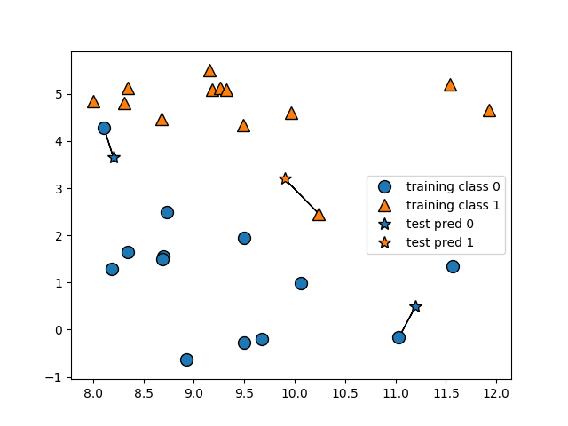
Moreover, we can now visualise this using mglearn:
mglearn.plots.plot_knn_classification(n_neighbors=1)
plt.show()
n_neighbors = 5
Now, what happens if we decide to use 5 nearest neighbors? Let’s find out!
knn = KNeighborsClassifier(n_neighbors=5)
knn.fit(x_train, y_train)

print("Training set score: {:.2f}".format(knn.score(x_train, y_train)))

print("Test set score: {:.2f}".format(knn.score(x_test, y_test)))
We now obtain a higher test set score of 0.94, with a slightly lower training set score of 0.95:
Training set score: 0.95
Test set score: 0.94
When we analyze this visually, we see that we now have 5 nearest neighbors for each test prediction instead of 1:
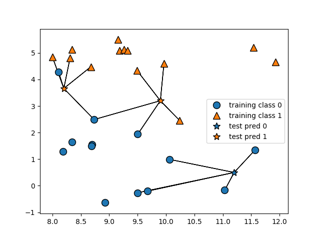
In this instance, we see that increasing the number of nearest neighbors increased the accuracy rate against our test data.
Cross Validation
One important caveat to note.
Given that we have used the train-test split method, there is always the danger that the split data is not random. i.e. the test data may be overly similar to the training data. This would mean that while the KNN model would demonstrate a high degree of accuracy on the training data, this would not necessarily be the case if new data was introduced outright.
In our case, given that the test set score is not that much lower than the training set score, this does not appear to be an issue here.
However, what method could we use to guard against this issue? The most popular one is a method called cross validation.
How Does Cross Validation Work?
Essentially, this works by creating multiple train-test splits (called folds) with the training data. Specifically, the algorithm is trained on k-1 folds while the final fold is referred to as the “holdout fold”, meaning that the final fold is used as the test set.
Let’s see how this works. In this particular instance, cross validation is unlikely to be of use to us here, since both the training and test set score was quite high on our original train-test split.
However, there are many instances where this will not be the case, and cross validation therefore becomes an important tool in splitting and testing our data more effectively.
For this purpose, suppose that we wish to generate 7 separate cross validation scores. We will first import our cross validation parameters from sklearn:
from sklearn.cross_validation import cross_val_score, cross_val_predict
Then, we generate 7 separate cross validation scores based on our prior KNN model:
scores = cross_val_score(model, x_scaled, y, cv=7)
print ("Cross-validated scores:", scores)
Here, we can see that the cross-validated scores do not increase as we add to the number of folds.
Cross-validated scores: [0.96402878 0.85611511 0.89855072 0.93478261 0.94202899 0.89051095 0.91240876]
This is expected since we still got quite a high test set score on our original train-test split.
With this being said, cross validation is quite commonly used when there is a large disparity between the training and the test set score, and the technique is quite useful under these circumstances. In other words, if we had a high training and low test set score, it becomes much more likely that the cross validation score would increase with each added fold.
Summary
In this tutorial, you have learned:
- What is a classification problem
- How KNN can be used to solve classification problems
- Configuring of data for effective analysis with KNN
- How to use cross validation to conduct more extensive accuracy testing
Many thanks for reading, and feel free to leave any questions in the comments below!