
MMS • RSS
Article originally posted on InfoQ. Visit InfoQ
Key Takeaways
- Hash tables are data structures that manage space, originally for a single application’s memory and later applied to large computing clusters.
- As hashing tables are applied to new domains, old methods for resizing hash tables have negative side effects.
- Amazon’s “Dynamo paper” of 2007 applied the consistent hashing technique to a key-value store. Dynamo-style consistent hashing was quickly adopted by Riak & Riak Core and other open source distributed systems.
- Riak Core’s consistent hashing implementation has a number of limits that cause problems when changing cluster sizes.
- Random Slicing is an extremely flexible consistent hashing technique that avoids all of Dynamo-style consistent hashing’s limitations.
This fall, Wallaroo Labs will be releasing a large new feature set to our distributed data stream processing framework, Wallaroo. One of the new features requires a size-adjustable, distributed data structure to support growing & shrinking of compute clusters. It might be a good idea to use a distributed hash table to support the new feature, but … what distributed hash algorithm should we choose?
The consistent hashing technique has been used for over 20 years to create distributed, size-adjustable hash tables. Consistent hashing seems a good match for Wallaroo’s use case. Here’s an outline of this article, exploring if that match really is as good as it seems:
- Briefly explain the problem that consistent hashing tries to solve: resizing hash tables without too much unnecessary work to move data.
- Summarize Riak Core’s consistent hashing implementation
- Point out the limitations of Riak Core’s hashing, both in the context of Riak and in terms of what Wallaroo needs in a consistent hashing implementation.
- Introduce the Random Slicing technique by example and with lots of illustrations
Introduction: The Problem: The Art of Resizing Hash Tables
Most programmers are familiar with hash tables. If hash tables are new to you, then Wikipedia’s article on Hash Tables is a good place to look for more detail. This section will present only a brief summary. If you’re very comfortable with hash tables, I recommend jumping forward to Figure 1 at the end of this section: I will be using several similar diagrams to illustrate consistent hashing scenarios later in this article.
A hash table is a data structure that organizes a computer’s memory. If we have some key called key, what part of memory is responsible for storing a value val that we want to associate with key?
Let’s borrow from that Wikipedia article for some pseudo-code:
let hash = some_hash_function(key)      ;; hash is an integer
let index = hash modulo array_size      ;; index is an integer
let val = query_bucket(key, index)      ;; val may be any data type
Hash tables usually have these three basic steps. The first two steps convert the key (which might be any data type) first into a big number (hash in the example above) and then into a much smaller number (index in the example). The second number is typically called the “bucket index” because hash tables frequently use arrays in their implementation. The index number is often calculated using modulo arithmetic.
Many types of hash table can store only a single value inside of a bucket. Therefore, the total number of buckets (array_size in the example above) is a very important constant. But if this size is constant, how can you resize a hash table? Well, it is “easy” if we allow array_size to be a variable instead of a constant. But if we continue using modulo arithmetic to calculate the index bucket number, then we have a problem whenever array_size changes.
Let’s look at the first 24 hash values, 0 through 23, as we change the number of buckets in our hash table from 3 to 10.
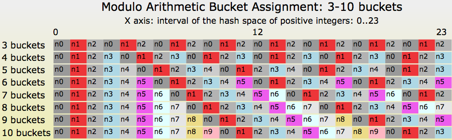
Figure 1: Illustration of modulo arithmetic to assign hash values to buckets
On the far left of Figure 1, the bucket assignments for hashes 0, 1, 2, and 3 do not change. But when the modulo arithmetic “rolls over” back to bucket 0, then everything changes. Can you see a red diagonal line that starts at (hash=4, buckets=3) and continues down and to the right? Most values to the right of that diagonal must move when we change the number of buckets!
The moving problem is usually worse as the new array_size grows, especially when array_size grows incrementally from N to N+1: only 1/N values will remain in the same bucket. We desire the opposite: we want only 1/N values to move to a new bucket.
Consistent hashing is one way to give us very predictable hash table resizing behavior. Let’s look at a specific implementation of consistent hashing and see how it reacts to resizing.
A Tiny Sliver of the History of Consistent Hashing and Riak Core
A traditional hash table is a data structure for organizing space: computer memory. In 1997, staff at Akamai published a paper that recommended using a hash table to organize a different kind of space: a cluster of HTTP cache servers. This widely influential paper was “Consistent Hashing and Random Trees: Distributed Caching Protocols for Relieving Hot Spots on the World Wide Web”.
Amazon published a paper at SOSP 2007 called “Dynamo: Amazon’s Highly Available Key-value Store”. Inspired by this paper, the founders of Basho Technologies, Inc. created the Riak key-value store as an open source implementation of Dynamo. Justin Sheehy made one of the first public presentations about Riak at the NoSQL East 2009 conference in Atlanta.. The Riak Core library code was later split out of the Riak database and can be used as a standalone distributed system platform.
Earlier this year (2018), Damian Gryski wrote a blog article that caught my eye and that I recommend for presenting alternative implementations & comparisons of consistent hashing functions: ”Consistent Hashing: Algorithmic Tradeoffs”.
Riak Core’s Consistent Hashing algorithm
A lot has been written about the consistent hashing algorithm used by Riak Core. I’ll present a summary-by-example here to prepare for a discussion later of Riak Core’s hashing limitations.
I’ll borrow a couple of diagrams from Justin Sheehy’s original presentation. The first diagram is a hash ring with 32 partitions and 4 nodes assigned to various parts of the ring. Riak Core uses the SHA-1 algorithm for hashing strings to integers. SHA-1’s output size is 160 bits, which can be directly mapped onto the integer range 0..2160-1.
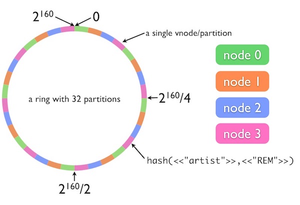
Figure 2: A Riak Ring with 32 partitions and interval claims by 4 nodes
Riak Core’s data model splits its namespace into “buckets” and “keys”, which are not exactly the same definitions that I used in the last section. This example uses the Riak bucket name “artist” and Riak key name “REM”. Those two strings are concatenated together and used as the input to Riak Core’s consistent hash function.
This example’s hash ring is divided into 32 partitions of equal size. Each of the four server nodes is assigned 8 of the 32 partitions. In this example, the string “artist” + “REM” maps via SHA-1 to a position on the ring at roughly 4 o’clock. The pink node, node3, is assigned to this section of the ring. If we ignore data replication, then we say that node3 is the server responsible for storing the value of the key “artist” + “REM”.
Our second example adds data replication. What happens if node3 has crashed? How can we locate other replicas that store our key?
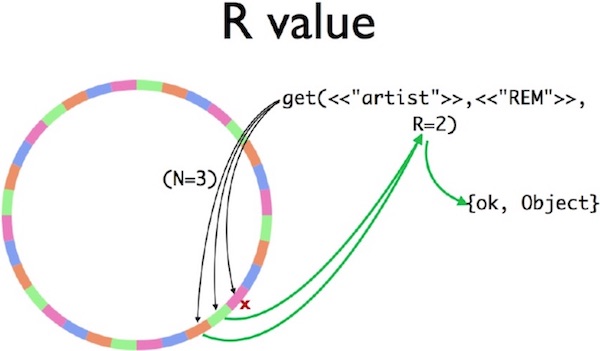
Figure 3: A Riak get query on a 32 partition ring
Riak Core uses several constants to help describe where data replicas are stored. Two of these constants are N, the total number of value replicas per key, and R, the minimum number of successful server queries needed to fetch a key from the database. To calculate the set of all servers that are responsible for a single key, the hash algorithm “walks around the ring clockwise” until N unique servers have been found. In this example, the replica set is handled by pink, green, and orange servers (i.e., node3, node0, and node1)
This second diagram shows that the pink server (node3) has crashed. A Riak Core client will send its query to N=3 servers. No reply is sent by node3. But the replies from node0 and node1 are sufficient to meet the R=2 constraint; the client responds with an {ok,Object} successful reply.
The Constraints and Limits of Riak Core’s Consistent Hashing algorithm
I worked for Basho Technologies, Inc. for six years as a senior software engineer. My intent in this section is a gentle critique, informed by hindsight and discussion with many former Basho colleagues. While at Basho, I supported keeping what I can call now limits or even flaws in Riak Core: they all were sensible tradeoffs, back then. Today, we have the benefit of hindsight and time to reflect on new discoveries by academia and industry. Basho was liquidated in 2017, and its source code assets were sold to UK-based Bet365. Riak Core’s maintenance continues under Bet365’s ownership and by the Riak open source community.
Here’s a list of the assumptions and limits of Riak Core’s implementation of the Dynamo-style consistent hashing algorithm. They are listed in roughly increasing order of severity, hassle, and triggers for Customer Support tickets and escalations at Basho Technologies, Inc.
- The only string-to-integer hash algorithm is SHA-1.
- The hash “rings” integer interval is the range 0 to 2^160-1.
- The number of partitions is fixed.
- The number of partitions must be a power of 2.
- The size of each partition is fixed.
- Historically, the “claim assignment” algorithm used to assign servers to intervals on the ring were buggy and naive and frequently created imbalanced workload across nodes.
- Server capacity adjustment by “weighting” did not exist: all servers were assumed equal.
- No support for segregating extremely “hot” keys, for example, Twitter’s “Justin Bieber” account.
- No effective support for “rack-aware” or “fault domain aware” replica placement policy
Limits 1 and 2 are quite minor, both being tied to the use of the SHA-1 hash algorithm. The effective hash range of 160 bits was sufficient for all Riak use cases that I’m aware of. There were a handful of Basho customers who wanted to replace SHA-1 with another algorithm. The official answer by Basho’s Customer Support staff was always, “We strongly recommend that you use SHA-1.”
I believe that limits 3-5 made sense, once upon a time, but they should have been eliminated long ago. The original reason to keep those limits was,“Dynamo did it that way.” Later, the reason was, “The original Riak code did it that way.” After the creation of the Riak Core library, the reason turned into, “It is legacy code that nobody wants to touch.” The details why are a long diversion away from this article, my apologies.
Limits 6-9 caused a lot of problems for Basho’s excellent Customer Support Engineers as well as for Basho’s developers and finally into Basho’s marketing and business development. Buggy “claim assignment” (limit #6) could cause terrible data migration problems if moving from X number of servers to Y servers, for some unlucky pairs of X and Y. Migrating old Riak clusters from older & slower hardware to newer & faster machines (limit #7) was difficult when the ring assignments assumed that all machine had the same CPU & disk capacity; manual workarounds were possible, but Basho’s support staff were almost always involved in each such migration.
Riak Core is definitely vulnerable to the “Justin Bieber” phenomenon (limit #8): a “hot” key that gets several orders of magnitude more queries than other keys. The size of a Riak Core partition is fixed: any other key in the same partition as a super-hot key would suffer from degraded performance. The only mitigation was to migrate to a ring with more partitions (which violated constraint #3 but was actually feasible via a manual procedure (and help from Basho support) and then also manually reassign the hot key partition (and the servers clockwise around the ring) to larger & faster machines.
Limit #9 was a long-term marketing and business expansion problem. Riak Core usually had little problem maintaining N replicas of each object. As an eventually-consistent database, Riak would err conservatively and make more than N replicas of an object, then copy and merge together replicas in an automatic “handoff” procedure.
However, the claim assignment had no support for “rack awareness” or “fault domain awareness”, where a failure of a common power supply, network router, or other common infrastructure could cause multiple replicas to fail simultaneously. A replica choice strategy of “walk clockwise around the ring” could sometimes be created manually to support a single static data center configuration, but as soon as the cluster was changed again (or if a single server failed), then the desired replica placement constraints would be violated.
Dynamo’s and Riak Core’s consistent hashing: a retrospective
The 2007 Dynamo paper from Amazon was very influential. Riak adopted its consistent hashing technique and still uses it today. The Cassandra database uses a close variation. Other systems have also adopted the Dynamo scheme. As an industry practitioner, it is a fantastic feeling to read a paper and think, “That’s a great idea,” and “I can easily write some code to do that.” But it is also a good idea to look into the rear view mirror of time and experience and ask, “Is it still a good idea?”
While at Basho Technologies, I maintained, supported, and extended many of Riak’s subsystems. I think Riak did a lot of things right in 2009 and still does a lot of things right in 2018. But Riak’s consistent hashing is not one of them. The limits discussed in the previous section caused a lot of real problems that are (with the benefit of hindsight!) avoidable. Many of those limits have their roots in the original Dynamo paper. As an industry, we now have lots of experience from Basho and from other distributed systems in the open source world. We also have a decade of academic research that improves upon or supersedes Dynamo entirely.
Wallaroo Labs decided to look for an alternative hashing technique for Wallaroo. The option we’re currently using is Random Slicing, which is introduced in the second half of this article.
Random Slicing: a Different Consistent Hashing Technique
An alternative to Riak Core’s consistent hashing technique is Random Slicing. Random Slicing is described in “Random Slicing: Efficient and Scalable Data Placement for Large-Scale Storage Systems” by Miranda et al. in 2014. The important difference with Riak Core’s technique are:
- Any hash function that maps string (or byte list or byte array) to integers or floating point numbers may be used.
- The visual model of the hash space as a ring is not needed: replica placement is not determined by examining neighboring partitions of the hash space.
- The hash space may have any number of partitions.
- A partition of the hash space may be any size greater than zero.
These differences are sufficient to eliminate all of the weaknesses of Riak Core’s consistent hashing algorithm, in my opinion. Let’s look at several example diagrams to get familiar with Random Slicing, then we will re-examine Riak Core’s major pain points that I described in the previous section.
Let’s first look at some possible Random Slicing map illustrations that involve only 3 nodes.
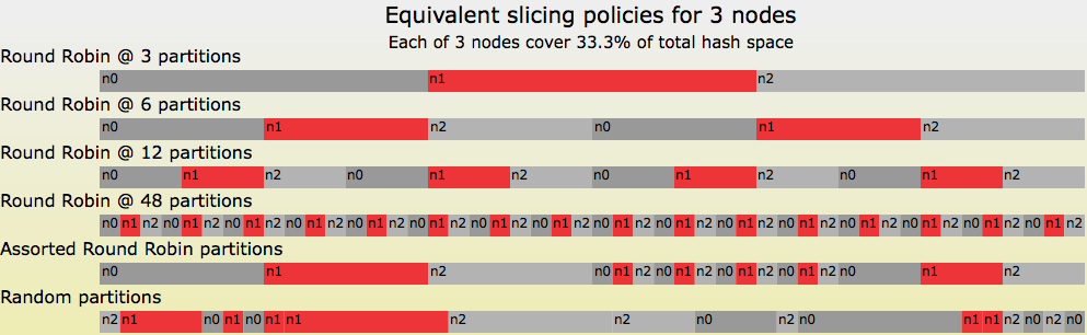
Figure 4: Six equivalent Random Slicing policies for a 3 node map
In all six cases in Figure 4, the amount of hash space assigned to n0, n1, and n2 is equal to 33.3%. The top case is simplest: each node is assigned a single contiguous space. Cases 2-4 look very similar to Riak Core’s initial ring claim policy, though without Riak Core’s power-of-2 partition restriction. Case 5, “Assorted Round Robin Partitions”, is actually a combination of earlier cases: case 2 for intervals in 0%-50%, case 4 for intervals in 50%-75%, and case 3 for intervals in 75%-100%. The bottom case is a random sorting of case 4’s intervals: note that there are three cases where nodes are assigned adjacent intervals!
Evolving Random Slicing Maps Over Time
All of the cases in Figure 4 are valid Random Slicing policies for a single point in time for a hash map. Let’s now look at an example of re-sizing a map over time (downward on the Y-axis) in Figure 5.
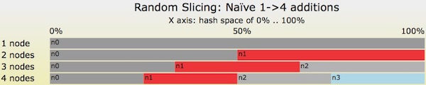
Figure 5: A naïve example of re-sizing a Random Slicing map from 1-> 4 nodes.
Figure 5 is terrible. I don’t recommend that anybody use Random Slicing in this way. I’ve included this example to make a point: there are sub-optimal ways to use Random Slicing. In this example, when moving from 1->2 nodes, 2->3 nodes, and 3->4 nodes, the total amount of keys moved in the hash space is equal to about 50.0 + (16.7 + 33.3) + (8.3 + 16.6 + 25.0) = 150%. That’s far more data movement than an optimal solution would provide.
Let’s look at Figure 6 for an optimal transition from 1->4 nodes and then go one step further with a re-weighting operation.
- Start with a single node,
n0. - Add node
n1with weight=1.0 - Add node
n2with weight=1.0 - Add node
n3with weight=1.0 - Change
n3’s weight from 1.0 -> 1.5. For example, noden3got a disk drive upgrade with 50% larger capacity than the other nodes.

Figure 6: A series of Random Slicing map transitions as 1->4 nodes are added then n3’s weight is increased by 50%
After step 4, when all 4 nodes have been added with equal weight, the total interval assigned to each node is 25%: ‘n0’ is assigned a single range of 25%, and ‘n3’ is assigned three ranges of 8.33% adds up to 25%. The amount of data migrated by each step individually and in total is optimal: 50.0% + 33.3% + 25.0% = 108.3%. When compared to the bad example of Figure 5, the steps in Figure 6 will avoid a substantial amount of data movement!
After step 5, which changes the weighting factor of node n3 from 1.0 to 1.5, the amount of hash space assigned to ‘n3’ grows from 25.0% to 33.3%. The other three nodes must give up some hash space: each shrinks from 25.0% to 22.2%. The ratios of assigned hash spaces is exactly what we desire: 33.3% / 22.2% = 1.5.
Finally, let’s look at a transition diagram in Figure 7. It starts with 4 nodes in the Random Slicing map. We then add 3 servers each, four times in a row. At the end, the Random Slicing maps will contain 16 nodes. Let’s see what the maps look like using three different techniques: Riak Core’s consistent hashing, Random Slicing with an optimal slicing strategy, and the naïve contiguous strategy.
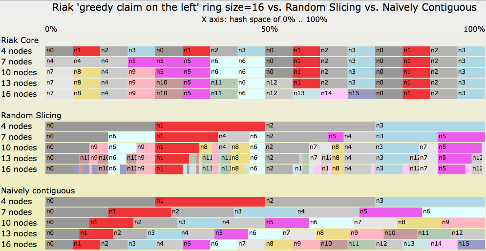
Figure 7: Transitions from 4->7->10->13->16 nodes by three different slicing strategies
Some notes about Figure 7:
- The “Naïvely Contiguous” strategy at the bottom ends each transition with perfectly balanced assignments of hash space to each node. However, it causes a huge amount of unnecessary data movement during each transition.
- The Riak Core strategy at the top is optimal in terms of data migration by each transition, but the amount of hash space assigned to individual nodes is often unbalanced.
- Two cases of balance: in 4 & 16 node cases, all nodes are assigned an equal amount of hash space, 25.0% and 6.25%, respectively.
- Three cases of imbalance: 7, 10, and 13 nodes.
- In the 7 node case, nodes
n4andn5are assigned 3 partitions when the other nodes are assigned 2 partitions. The imbalance factor is 1.5. - In the 10 & 13 node cases, nodes
n0, n1, n2,andn3are assigned 2 partitions when some other nodes are assigned 1 partition. The imbalance factor is 2.0.
- The strategy in the middle is optimal both in terms of node balance after each transition and also the amount of data moved during each transition.
Random Slicing and Super-Hot “Justin Bieber Keys”
Let’s start with the Random Slicing perfect strategy in the middle of Figure 7, with 4 nodes in the map. Then let’s assume that the super-hot key for our Justin Bieber customer hashes to exactly 6.00000% in the hash space. In all phases of Figure 7, 6% is mapped to node n0. We know that n0 cannot handle all of the load for the Justin Bieber key and also all other keys assigned to it.
However, random slicing allows us the flexibility to create a new, very thin partition from 6.00000% to 6.00001% and assign it to node n11, which is the fastest Cray 11 super-ultra-computer that money can buy. Problem solved!
Maybe we solved it, but maybe we didn’t. In the real world, the Cray 11 does not exist. But if we could use a flexible placement policy, we can solve our Justin Bieber problem.
Random Slicing and Placement Policy Flexibility
There is one weakness in Riak Core’s consistent hashing that hasn’t been addressed yet by the Random Slicing technique: placement policy. But that is easy to fix. We’ll just add a level of indirection! (Credit to David Wheeler, see Wikipedia’s “Indirection” topic.)
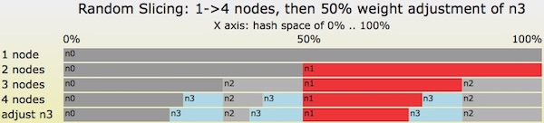
Figure 6 (again): A series of Random Slicing map transitions as 1->4 nodes are added then n3’s weight is increased by 50%
Let’s look at Figure 6 again. Figure 6 gives us a mapping from a hash space interval to a single node or single machine. Instead, we can introduce a level of indirection at this point, mapping instead from a hash space interval to a replica placement policy. Then we can define any placement policy that we wish. For example:
- Node
n0-> Policy 0: store with Paxos replicated state machines on nodes 82, 17, and 22. - Node
n1-> Policy 1: store with Chain Replication state machines on nodes 77 and 23. - Node
n2-> Policy 2: use 7+2 Reed-Solomon erasure coding striped across nodes 31-39. - Node
n3-> Policy 3: send the data to the color printer in San Francisco - Node
n11-> Policy 11: use a special cluster of 81 primary/secondary replica machines: the 1 primary to handle updates as Justin changes stuff, and 80 read-only cache machines to handle the workload caused by Justin’s enthusiastic fans.
What Does a Random Slicing Implementation Look Like?
Let’s take a look at the data structure(s) needed for Random Slicing, considerations for partition policies, and what Random Slicing cannot do on its own.
Random Slicing implementation: data structures
If you needed to write a Random Slicing library today, one way to look at the problem is to consider major constraints. Some constraints to consider might be:
- How quickly do I need to execute a single range query, i.e., start with a key such as a string or a byte array and end with a Random Slicing partition?
- Related: How many partitions do I expect the Random Slicing map to hold?
- How much RAM am I willing to trade for that speed?
- What kind of information do I need to store with the Random Slicing partition? Am I mapping to a single node name (as a string or an IP address or something else?), or to a more general placement policy description?
Constraint A will drive your choice of a string/byte array -> integer hash function as well as the data structure used for range queries. For the former, will a crypto hash function like SHA-1 be fast enough? For the latter, will you need a search speed of O(1) in the partition table, or is something like O(log(N)) alright, where N is the number of partitions in the table?
Together with constraint B, you’re most of the way to deciding what data structure to use for the range query. The goal is: given an integer V (the output value from my standard hash function, e.g., SHA-1), what is the Random Slicing partition (I,J) such that I <= V < J. If you have easy access to an interval tree library, your work is nearly done for you. The same if you have a balanced tree library that can perform an “equal or less than” query: insert all of the lower bound values I into the tree, then perform an equal or less than query for V. Some trie libraries also include this type of query and may have a good space vs. time trade-off for your application.
If you need to write your own code, one strategy is to put all of the lower bounds values I into a sorted array. To perform the equal or less than query, use a binary search of the array to find the desired lower bound. This is the approach that we’re prototyping now with Wallaroo, written in the Pony language.
class val HashPartitions
    let _lower_bounds: Array[U128] = _lower_bounds.create()
    let _lb_to_c: Map[U128, String] = _lb_to_c.create()
- The initial hash function is MD5, which is fast enough for our purposes and has a convenient 128-bit output value. Pony has native support for unsigned 128-bit integer data and arithmetic.
- The data structures shown above (code link) uses an array of
U128unsigned 128-bit integers to store the lower bound of each partition interval. - The lower bound is found with a binary search (code link) over the
_lower_boundsarray. - The lower bound integer is used as a key to a Pony map of type
Map[U128, String], which uses aU128typed integer as its key and returns aStringtyped value.
In the end, we get a String data type, which is the name of the Wallaroo worker process that is responsible for the input key. If/when we need to support more generic placement policies, the String type will be changed to a Pony object type that will describe the desired placement policy. Or perhaps it will return an integer, to be used as an index into an array of placement policy objects.
In contrast, Riak Core uses its limitations of fixed size and power-of-2 partition count to simplify its data structure. Given a ring size S, the upper log2(S) bits of the SHA-1 hash value are used for an index into an array of S partition descriptors.
Random Slicing implementation: partition placement (where to put the slices?)
The data structures needed for Random Slicing are quite modest. As we saw earlier in the examples in Figure 4 and Figure 7, much of Random Slicing’s benefits come from clever placement & sizing of the hash partitions. What algorithm(s) should we use?
The Random Slicing paper by Miranda and collaborators, is an excellent place to start. Some of the algorithms and strategies used to solve “bin packing” problems can be applied to this area, although standard bin packing doesn’t allow you to change the size or shape of the items being packed into the bin.
From a practical point of view, if a Random Slicing map is added to frequently enough, then it’s possible to create partitions so thin that they cannot be represented by the underlying data structure. In code that I’d written a few years ago for Basho (but not used by Riak), the underlying data structure used floating point numbers between 0.0 and 1.0. After adding a single node to a map, one at a time, then after repeating several dozen more times, a partition can become so thin that a double floating point variable can no longer represent the interval.
When it becomes impossible to slice a partition, then some partitions must be reassigned: coalesce many tiny partitions into a few larger partitions. Any such reassignment requires moving data, for “no good reason” other than to make partition slicing possible again. There’s a rich space for solving optimization problems here, to choose the smallest intervals in such a way to minimize the total sum of intervals reassigned while maximizing the benefit of creating larger contiguous partitions. Or perhaps you solve this problem another way: to upgrade your app to use a different data structure that has a smaller minimum partition size, then deal with the hassle of upgrading everything. Either approach might be the best one for you.
Random Slicing implementation: out-of-bounds topics
If we use the right data structures and write all the code to implement a Random Slicing map, then we’ve solved all our application’s distributed data problems, haven’t we? I’d love to say yes, but the answer is no. Some other things you need to do are:
- Distribute copies of the Random Slicing map itself, probably with some kind of version numbering or history-preserving scheme.
- Move your application’s data when the Random Slicing map changes.
- Deal with concurrent access to your app’s data while its location while it is being moved.
- Manage all of the data races that problems 1-3 can create.
Random Slicing cannot solve any of these problems. Nor is there a single solution to the equation of your-distributed-application + Random-Slicing = new-resizable-distributed-application. Solutions to these problems are application-specific.
Conclusion: Random Slicing is a Big Step Up From Riak Core’s Hashing
I hope you’ll now believe my claims that Random Slicing is a far more flexible and useful hashing method than Riak Core’s consistent hashing. Random Slicing can provide fine-grained load balancing across machines while minimizing data copying when machines are added, removed, or re-weighted in the Random Slicing map. Random Slicing can be easily extended to support arbitrary placement policies. The problem of extremely hot “Justin Bieber keys” can be solved by adding very thin slices in a Random Slicing map to redirect traffic to a specialized server (or placement policy).
Wallaroo Labs will soon be using Random Slicing for managing processing stages within Wallaroo data processing pipelines. It is very important that Wallaroo be able to adjust workloads across participants without unnecessary data migration. We do not yet need multiple placement policies, but, if/when the time comes, it is reassuring that Random Slicing will make those policies easy to implement.
Online References
All URLs below were accessible in August 2018.
- Bet365. “Riak Core”.
- Decandia et al. “Dynamo: Amazon’s Highly Available Key-value Store”, 2007.
- Karger et al. “Consistent Hashing and Random Trees: Distributed Caching Protocols for Relieving Hot Spots on the World Wide Web”, 1997.
- Metz, Cade. “How Instagram Solved Its Justin Bieber Problem”, 2015.
- Miranda et al. “Random Slicing: Efficient and Scalable Data Placement for Large-Scale Storage Systems”, 2014.
- Sheehy, Justin. “Riak: Control your data, don’t let it control you”, 2009.
- Wallaroo Labs. “Wallaroo”.
- Wikipedia. “Hash Tables”.
- Wikipedia. “Indirection.”
About the Author
 Scott Lystig Fritchie was UNIX systems administrator for a decade before until switching to programming full-time at Sendmail, Inc. in 2000. While at Sendmail, a colleague introduced him to Erlang, and his world hasn’t been the same since. He has had papers published by USENIX, the Erlang User Conference, and the ACM and has given presentations at Code BEAM, Erlang Factory, and Ricon. He is a four-time co-chair of ACM Erlang Workshop series. Scott lives in Minneapolis, Minnesota, USA and works at Wallaroo Labs on a polyglot distributed system of Pony, Python, Go, and C.