
MMS • RSS
Article originally posted on Data Science Central. Visit Data Science Central
You won’t learn this in textbooks, college classes, or data camps. Some of the material in this article is very advanced yet presented in simple English, with an Excel implementation for various statistical tests, and no arcane theory, jargon, or obscure theorems. It has a number of applications, in finance in particular. This article covers several topics under a unified approach, so it was not easy to find a title. In particular, we discuss:
- When the central limit theorem fails: what to do, and case study
- Various original statistical tests, some unpublished, for instance to test if an empirical statistical distribution (based on observations) is symmetric or not, or whether two distributions are identical
- The power and mysteries of stable (also called divisible) statistical distributions
- Dealing with weighted sums of random variables, especially with decaying weights
- Fun number theory problems and algorithms associated with these statistical problems
- Decomposing a (theoretical or empirical / observed) statistical distribution into elementary components, just like decomposing a complex molecule into atoms
The focus is on principles, methodology, and techniques applicable to, and useful in many applications. For those willing to do a deeper dive on these topics, many references are provided. This article, written as a tutorial, is accessible to professionals with elementary statistical knowledge, like stats 101. It is also written in a compact style, so that you can grasp all the material in hours rather than days. This simple article covers topics that you could learn in MIT, Stanford, Berkeley, Princeton or Harvard classes aimed at PhD students. Some is state-of-the-art research results published here for the first time, and made accessible to the data science of data engineer novice. I think mathematicians (being one myself) will also enjoy it. Yet, emphasis is on applications rather than theory.
Finally, we focus here on sums of random variables. The next article will focus on mixtures rather than sums, providing more flexibility for modeling purposes, or to decompose a complex distribution in elementary components. In both cases, my approach is mostly non-parametric, and based on robust statistical techniques, capable of handling outliers without problems, and not subject to over-fitting.
1. Central Limit Theorem: New Approach
Let us consider a weighted sum of n independent and identically distributed random variables:
When the weights are identical, the central limit theorem (CLT) states that this converges to a Gaussian distribution. Regardless of the weights or n, we have:
 This is also true when n tends to infinity. Without loss of generality, we assume here that all these random variables have their expectation equal to 0. Now, let us decompose the weighted sum into two components. First, let us introduce a partition of N = {1, …, n} into two subsets I and J. For instance, the set I consists of the odd integers in N, and J consists of the even integers in N. Or I consists of the integers smaller than n/2, and J consists of the integers larger or equal to n/2. The decomposition is as follows:
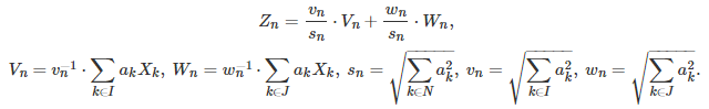
The variables Z(n), V(n) and W(n) have the same variance as X(1). Let us define p(n) = v(n) / s(n), and q(n) = w(n) / s(n). At the limit as n tends to infinity, assuming the limits exist, we have
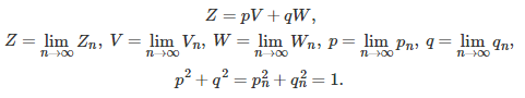
When the weights a(k)’s are identical (corresponding to the standard CLT) then the factors p and q can be made arbitrarily close to any real number (by choosing I and J appropriately) and thus the limit distribution satisfies the following property, presented here as a theorem:
Theorem
If the weights a(k) are identical (classic CLT framework) then Z can be written as any linear combination pV + qW of tho independent random variables V and W that have the same exact distribution as Z (with same variance), provided that p^2 + q^2 = 1.
Note that by convergence and limit, here we mean convergence in distribution. A distribution that satisfies the property stated in the above theorem, is called a stable distribution. Evidently the Gaussian distribution is one example of a stable distribution. But is it the only one? That is, does this property uniquely characterizes the Gaussian distribution?
Let us introduce the concept of semi-stable distribution. A random variable Z has a semi-stable distribution if for any strictly positive integer n, it can be written as the sum of n independent random variables, divided by SQRT(n), with each random variable having the same distribution as Z. Gaussian distributions are one example. All stable distributions are also semi-stable (see exercise below), but the converse might not be true.
Le’s say that the variables X(k) have a semi-stable distribution, but one that is non-Gaussian. For each value of n including at the limit as n tends to infinity, Z(n) would have (by construction) that exact same semi-stable distribution, which is non-Gaussian. But the central limit theorem states that at the limit, the distribution must be Gaussian. This contradiction makes you think that the only semi-stable distribution is the Gaussian one.
I won’t spend much time on this paradox, but I invite you to think about it. There are other stable and semi-stable distributions, as we shall see in the next section. Generally speaking, they have a thick tail and infinite variance.
Exercise
Prove that any stable distribution is also semi-stable. Hint: For a stable distribution, Z can be written as Z = SQRT(2/3) * { (V + W) / SQRT(2) } + SQRT(1/3) * U = (V + W + U) / SQRT(3), with U, V, W, (V + W) / SQRT(2) having the same distribution as Z. This easily generalizes to 4, 5 or more variables, and can be proved by induction. Here, U, V and W are independent.
2. Stable and Attractor Distributions
The initial problem I was interested in, is to approximate a random variable Z with a complicated distribution, by a weighted sum of independent, identically distributed random variables that have a simple distribution. These random variables, denoted as X(1), X(2) and so on throughout this article, are also called kernels.
We have seen that if if these kernels have a stable distribution, then Z must also have a stable (and identical) distribution. So, unless we want to restrict ourselves to the small family of stable distributions, we must consider unstable kernels. From now on, we will mostly focus on (unstable) kernels that have a uniform distribution.
The next question is: can any Z (regardless of its distribution) be represented (that is, decomposed) in this manner? It is similar to asking whether any real function can be represented by a Taylor series. The answer, in both cases, is no. The kind of random variables Z that can be represented in this manner are called attractors. Their distribution is called an attractor distribution. We are curious to find out
- which distributions can be attractors,
- whether Z‘s distribution depends on the choice of the kernels, and
- whether an attractor distribution must necessarily be a stable distribution, even if the kernel is not.
So clearly, we are here in a context where the assumptions of the CLT (central limit theorem) are violated, and the CLT does not apply. Let us introduce one additional notation: 
Depending on the weights a(k), the coefficient b(n,k) for any fixed k, may not depend on n, as n tends to infinity.
Using decaying weights
We shall consider, moving forward, decaying weights of the form a(k) = 1 / k^c, where c is a positive parameter in the interval [0.5, 1]. If c is less than or equal to 0.5, then we are back under the CLT conditions and Z has a Gaussian distribution, even if the kernel has a uniform distribution. If c is larger than 0.5, then we have the following:
- The distribution of Z is NOT a Gaussian one (see here for details.)
- For any fixed k, b(n, k) does not depend on n, as n tends to infinity. For instance, if c = 1, then b(n, k) tends to SQRT(6) * a(k) / Pi as n tends to infinity.
Decaying weights have plenty of applications. For instance, I used a decaying weighted sum of nearest neighbor distances in a k-NN clustering problems, rather than the k-th nearest neighbor alone, to boost robustness. The resulting distribution of Z was rather special; the details are available in this article.
More about stable distributions and their applications
In some sense, stable distributions are invariant under linear transformations, while semi-stable distributions are invariant under addition. The Wikipedia entry for stable distributions is worth reading, especially the section related to the CLT. Examples of stable distributions, besides the Gaussian one, include the Levy and Cauchy distributions; both of them have infinite variance. Stable distributions are also related to the Levy process, with applications to financial markets.
The following references provide additional insights about the topics discussed here:
- Limit Distributions for Sums of Independent Random Variables (book published in 1954; costs $686 on Amazon, though I bought it for under $50 an hour ago — it must be the last copy)
- Table of content, for previous book
- Random Summation: Limit Theorems and Applications (1996; costs $245 on CRC Press)
- Random Summation: Limit Theorems and Applications (same book, this time on Amazon; costs $41)
3. Non CLT-compliant Weighted Sums, and their Attractors
In this section, we investigate what happens when using decaying weights a(k) = 1 / k^c, with c = 1, and with uniform kernels on [-0.5, 0.5], as discussed in the previous section. The busy reader can jump to to the conclusion at the bottom. For the statistician, data scientist, or machine learning architect, I present simple, interesting statistical tests that were used during my analysis, to obtain my results and conclusions.
Testing for normality
In our main test, we divided N = {1, …, n} into two subsets I and J as follows: I contains the integers less than 20; and J the integers greater or equal to 20. We also tested other partitions of N, see tests for semi-stability, below. Here, n was set to 100. We sampled from 5 different distributions, generating m = 20,000 deviates for each one:
- A Gaussian distribution for comparison purpose (Gaussian A)
- Another Gaussian distribution (Gaussian B) to assess variations across two samples from a same distribution
- X(n), Y(n), and Z(n)
The testing was done in Excel. By construction, all these distributions have a theoretical mean and median equal to zero, and a variance equal to 1/12 (that’s the variance of the kernel), as evidenced by the estimates in the table below. The number P.80 represents the 80th percentile. The number P.25 + P.75 is zero if the distribution is symmetric. This is the case in this example.
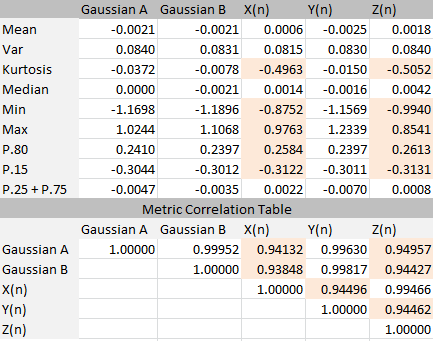
The sample size (m = 20,000) gives about two correct decimals in the table. The rule of thumb is that the precision is equal to about 1 / SQRT(m) except for Max and Min, which are always highly volatile. Clearly, the two Gaussian A and B look identical as expected, the distribution of X(n) and Z(n) look identical too though clearly non Gaussian, and the distribution of Y(n) look Gaussian. In fact it is not Gaussian, but close: the sample size is too small to pinpoint the difference. Likewise, X(n) and Y(n) do not have the same exact distribution (almost) but the sample size is too small to pinpoint the difference. This framework actually serves as a great benchmark to assess the power of the statistical tests involved.
We also performed visual tests to measure the difference between pairs of percentile distributions, see figure below.
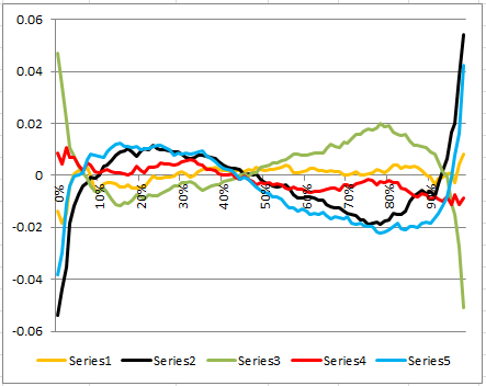
The yellow curve shows the empirical (observed) percentiles delta between the two Gaussian A and B. The differences are negligible. The red curve shows the percentile delta between the (almost identical) distributions of X(n) and Z(n). To the contrary, the three other curves are comparing distributions that are significantly different. For instance, the black curve represents the difference between Gaussian A and the distribution of X(n). These percentile tests are similar to a Kolmogorov-Smirnov test, except that Kolmogorov-Smirnov is based on the empirical cumulative distribution (CDF) while ours is based on the empirical percentile function, which is the inverse of the CDF. They clearly show when distributions are statistically different.
All the Excel computations are available in this spreadsheet. Look at the first tab labeled “Uniform”.
Testing for symmetry and dependence on kernel
One can compare R(x) = | 2 * Median – P.x – P.(1-x) | with that of a symmetric distribution, for various values of x between 0 and 0.5, to check if a distribution is symmetric around the median. The theoretical value of R(x) is zero regardless of x, if your empirical distribution is symmetric. Here P.x represents the x-th percentile.
In this test, we used a highly non-symmetric kernel: a mixture of Bernoulli and uniform distributions. We discovered that while the limit (attractor) distribution is much less asymmetric than the kernel, it is still clearly non symmetric. This also means that the distribution of Z depends on the kernel: when the kernel has a symmetric distribution, Z also has a symmetric distribution.
Testing for semi-stability
As stated in the first section, if the limiting distribution is semi-stable, it must satisfy Z = pV + qW, with p = q = 1 / SQRT(2). I tried various combinations for the subsets of indices I and J, but could not get close to p = q. Indeed, the closest you can get is with I = {1} and J = {2, 3, …, n}. When n tends to infinity, this leads to p = 0.78 and q = 0.63 (approximately); the exact values are p = SQRT(6) / Pi and q = SQRT(Pi^2 – 6) / Pi.
If you try a(k) = 1 / k^c, with c = 0.6 rather than c = 1, you might be able to get p = q with a judicious choice of I and J. Likewise, if you try with a(k) = 1 / (k+5) rather than a(k) = 1 / k, it might work. However the resulting Z, V and W still have different distributions, so it fails to prove that Z is semi-stable.
So how do you choose I and J to get p = q, assuming this equality is reachable in the first place? Whether or not it is feasible depends on how fast the weights decay. This is actually a number theory problem. For instance, if n = 18, a(k) = 1 / (k+5), I = {1, 4, 6, 8, 10, 12, 14, 15, 18} and J = {2, 3, 5, 7, 9, 11, 13, 16, 17}, then we get very close to p = q. This configuration was obtained using a greedy algorithm, as described fox example in this article.
Conclusions
The framework discussed here produces a Gaussian distribution as the limit distribution for the weighted sum, if the weights are decaying slowly. This is just the standard CLT. If the weights are decaying a bit too fast — faster than 1 / SQRT(k) but not faster than 1 / k — the following issues and benefits arise:
- The limiting distribution (attached to Z) is not Gaussian: good, that is what we were looking for.
- The limiting distribution (also called attractor) is not stable either, offering more flexibility. It may not even be symmetrical.
- Few distributions can be an attractor, so the amount of flexibility offered with fast-decaying weights is still limited. In fact, attractors don’t look very much different from Gaussian distributions, though they are clearly not Gaussian; this offers limited possibilities for modeling.
- The limiting distribution depends both on the choice for the kernel, and the first few terms in the weighted sum, unlike with the classic CLT; it is a mixture of a normal distribution, with a non-normal distribution. The non-normal part is attached to the first few terms of the weighted sum. This is indeed not bad, as it allows you to decompose these sums into two parts: the sum of the first 10 terms or so (non-normal) and the remaining of the sum (almost normal.) This is helpful for modeling purposes, allowing you to separate background noise (Gaussian-like tail) from the true signal.
A better tool to decompose a potential attractor into an infinite collection of basic kernels, is a mixture model, rather than a weighted sum. In that case, any distribution can be an attractor. This will be discussed in my next article, and it has plenty of applications.
For related articles from the same author, click here or visit www.VincentGranville.com. Follow me on on LinkedIn, or visit my old web page here.
DSC Resources
- Invitation to Join Data Science Central
- Free Book: Applied Stochastic Processes
- Comprehensive Repository of Data Science and ML Resources
- Advanced Machine Learning with Basic Excel
- Difference between ML, Data Science, AI, Deep Learning, and Statistics
- Selected Business Analytics, Data Science and ML articles
- Hire a Data Scientist | Search DSC | Classifieds | Find a Job
- Post a Blog | Forum Questions