
MMS • RSS
Article originally posted on Data Science Central. Visit Data Science Central
Though CNNs have mostly been used for computer vision tasks, nothing stops them from being used in NLP applications. One such application for which CNNs have been used effectively is sentence classification.
In sentence classification, a given sentence should be classified to a class. We will use a question database, where each question is labeled by what the question is about. For example, the question, “Who was Abraham Lincoln?” will be a question and its label will be Person.
We will use the CNN network introduced in the paper by Yoon Kim, Convolutional Neural Networks for Sentence Classification, to understand the value of CNNs for NLP tasks.
CNN structure
Now we will discuss the technical details of the CNN used for sentence classification. First, we will discuss how data or sentences are transformed to a preferred format that can easily be dealt with by CNNs. Next, we will discuss how the convolution and pooling operations are adapted for sentence classification, and finally, we will discuss how all these components are connected.
You can find the code to follow with this article.
Data transformation
Let’s assume a sentence of p words. First, we will pad the sentence with some special word (if the length of the sentence is < n) to set the sentence length to n words, where n≥p. Next, we will represent each word in the sentence by a vector of size k, where this vector can either be a one-hot-encoded representation, or Word2vec word vectors learnt using skip-gram, CBOW, or GloVe. Then a batch of sentences of size b can be represented by a b×n×k matrix.
Let’s walk through an example. Let’s assume the following three sentences:
- Bob and Mary are friends.
- Bob plays soccer.
Mary likes to sing in the choir.
In this example, the third sentence has the most words, so let’s set n=7, which is the number of words in the third sentence. Next, let’s assume the one-hot-encoded representation for each word. In this case, there are 13 distinct words. Therefore, we get this:
Bob: 1,0,0,0,0,0,0,0,0,0,0,0,0
and: 0,1,0,0,0,0,0,0,0,0,0,0,0
Mary: 0,0,1,0,0,0,0,0,0,0,0,0,0
Also, k=13 for the same reason. With this representation, we can represent the three sentences as a three-dimensional matrix of size 3×7×13, as shown in Figure 1:

Figure 5.1: A sentence matrix
The convolution operation
If we ignore the batch size, that is, if we assume that we are only processing a single sentence at a time, our data is a n×k matrix, where n is the number of words per sentence after padding, and k is the dimension of a single word vector. In our example, this would be 7×13.
Now we will define our convolution weight matrix to be of size m×k, where m is the filter size for a one-dimensional convolution operation. By convolving the input x of size n×k with a weight matrix W of size m×k, we will produce an output of h of size 1×n as follows:
Here, wi,j is the (i,j)th element of W and we will pad x with zeros so that h is of size 1×n. Also, we will define this operation more simply, as shown here:
Here, * defines the convolution operation (with padding) and we will add an additional scalar bias b. Figure 2 illustrates this operation:

Figure 2: A convolution operation for sentence classification
Then, to learn a rich set of features, we have parallel layers with different convolution filter sizes. Each convolution layer outputs a hidden vector of size 1×n, and we will concatenate these outputs to form the input to the next layer of size q×n, where q is the number of parallel layers we will use. The larger that q is, the better is the performance of the model.
The value of convolving can be understood in the following manner. Think about the movie rating learning problem (with two classes, positive or negative), and we have the following sentences:
I like the movie, not too bad
I did not like the movie, bad
Now imagine a convolution window of size 5. Let’s bin the words according to the movement of the convolution window:
The sentence I like the movie, not too bad gives:
[I, like, the, movie, ‘,’]
[like, the, movie, ‘,’, not]
[the, movie, ‘,’, not, too]
[movie, ‘,’, not, too, bad]
The sentence I did not like the movie, bad gives the following:
[I, did, not, like, the]
[did, not ,like, the, movie]
[not, like, the, movie, ‘,’]
[like, the, movie, ‘,’, bad]
For the first sentence, windows such as the following convey that the rating is positive:
[I, like, the, movie, ‘,’]
[movie, ‘,’, not, too, bad]
However, in the second sentence, windows such as the following convey negativity in the rating:
[did, not, like, the, movie]
We are able to see such patterns that help to classify ratings, thanks to the preserved spatiality. For example, if you use a technique such as bag-of-words to calculate sentence representations that lose spatial information, the sentence representations would be highly similar. The convolution operation plays an important role in preserving spatial information of the sentences.
Having q different layers with different filter sizes, the network learns to extract the rating with different size phrases, leading to an improved performance.
Pooling over time
The pooling operation is designed to subsample the outputs produced by the previously discussed parallel convolution layers. This is achieved as follows.
Let’s assume the output of the last layer h is of size q×n. The pooling over time layer would produce an output h’ of size q×1 output. The precise calculation would be as follows:
Here, h(i)=W(i)*x+b and h(i) is the output produced by the ith convolution layer and W(i) is the set of weights belonging to that layer. Simply put, the pooling over time operation creates a vector by concatenating the maximum element of each convolution layer. We will illustrate this operation in Figure 3:
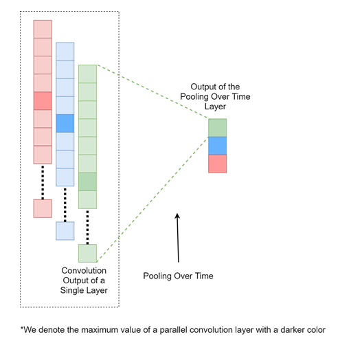
Figure 3: The pooling over time operation for sentence classification
By combining these operations, we finally arrive at the architecture shown in Figure 4:

Figure 4: A sentence classification CNN architecture
Implementation – sentence classification with CNNs
First, we will define the inputs and outputs. The input will be a batch of sentences, where the words are represented by one-hot-encoded word vectors—word embeddings will deliver even better performance than the one-hot-encoded representations; however, we will use the one-hot-encoded representation for simplicity:
sent_inputs = tf.placeholder(shape=[batch_size,sent_length,vocabulary_size],dtype=tf.float32,name=’sentence_inputs’)
sent_labels = tf.placeholder(shape=[batch_size,num_classes],dtype=tf.float32,name=’sentence_labels’)
Here, we will define three different one-dimensional convolution layers with three different filter sizes of 3, 5, and 7 and their respective biases:
w1 = tf.Variable(tf.truncated_normal([3,vocabulary_size,1],stddev=0.02,dtype=tf.float32),name=’weights_1′)
b1 = tf.Variable(tf.random_uniform([1],0,0.01,dtype=tf.float32),name=’bias_1′)
w2 = tf.Variable(tf.truncated_normal([5,vocabulary_size,1],stddev=0.02,dtype=tf.float32),name=’weights_2′)
b2 = tf.Variable(tf.random_uniform([1],0,0.01,dtype=tf.float32),name=’bias_2′)
w3 = tf.Variable(tf.truncated_normal([7,vocabulary_size,1],stddev=0.02,dtype=tf.float32),name=’weights_3′)
b3 = tf.Variable(tf.random_uniform([1],0,0.01,dtype=tf.float32),name=’bias_3′)
Now we will calculate three outputs, each belonging to a single convolution layer, as we just defined. This can easily be calculated with the tf.nn.conv1d function provided in TensorFlow. We use a stride of 1 and zero padding to ensure that the outputs will have the same size as the input:
h1_1 = tf.nn.tanh(tf.nn.conv1d(sent_inputs,w1,stride=1,padding=’SAME’) + b1)
h1_2 = tf.nn.tanh(tf.nn.conv1d(sent_inputs,w2,stride=1,padding=’SAME’) + b2)
h1_3 = tf.nn.tanh(tf.nn.conv1d(sent_inputs,w3,stride=1,padding=’SAME’) + b3)
For calculating max pooling over time, we need to write the elementary functions to do that in TensorFlow, as TensorFlow does not have a native function that does this for us. However, it is quite easy to write these functions.
First, we will calculate the maximum value of each hidden output produced by each convolution layer. This results in a single scalar for each layer:
h2_1 = tf.reduce_max(h1_1,axis=1)
h2_2 = tf.reduce_max(h1_2,axis=1)
h2_3 = tf.reduce_max(h1_3,axis=1)
Then we will concatenate the produced outputs on axis 1 (width) to produce an output of size batchsize×q:
h2 = tf.concat([h2_1,h2_2,h2_3],axis=1)
Next, we will define the fully connected layers, which will be fully connected to the output batchsize×q produced by the pooling over time layer. There is only one fully connected layer in this case and this will also be our output layer:
w_fc1 = tf.Variable(tf.truncated_normal([h2_shape[1],num_classes],stddev=0.005,dtype=tf.float32),name=’weights_fulcon_1′)
b_fc1 = tf.Variable(tf.random_uniform([num_classes],0,0.01,dtype=tf.float32),name=’bias_fulcon_1′)
The function defined here will produce the logits that are then used to calculate the loss of the network:
logits = tf.matmul(h2,w_fc1) + b_fc1
Here, by applying the softmax activation to the logits, we will obtain the predictions:
predictions = tf.argmax(tf.nn.softmax(logits),axis=1)
Also, we will define the loss function, which is the cross-entropy loss:
loss = tf.reduce_mean(tf.nn.softmax_cross_entropy_with_logits_v2(labels=sent_labels,logits=logits))
To optimize the network, we will use a TensorFlow built-in optimizer called MomentumOptimizer:
optimizer = tf.train.MomentumOptimizer(learning_rate=0.01,momentum=0.9).minimize(loss)
Running these preceding defied operations to optimize the CNN and evaluate the test data as given in the exercise, gives us a test accuracy close to 90% (500 test sentences) in this sentence classification task.
It can be useful to know how the problem we just solved can be useful in the real world. Assume that you have a large document about the history of Rome in your hand, and you want to find about Julius Caesar without reading the whole document. In this situation, the sentence classifier we just implemented can be used as a handy tool to summarize the sentences that only correspond to a person, so you don’t have to read the whole document.
Sentence classification can be used for many other tasks as well; one common use of this is classifying movie reviews as positive or negative, which is useful for automating computation of movie ratings. Another important application of sentence classification can be seen in medical domain, which is extracting clinically useful sentences from large documents containing large amounts of text.
Summary
Here we end our discussion about using CNNs for sentence classification. We first discussed how one-dimensional convolution operations combined with a special pooling operation called pooling over time can be used to implement a sentence classifier based on the CNN architecture. Finally, we discussed how to use TensorFlow to implement such a CNN and saw that it in fact performs well in sentence classification.
You enjoyed an excerpt from Packt Publishing’s latest book Natural Language Processing with TensorFlow, written by Thushan Ganegedara. If you like writing modern natural language processing applications using deep learning algorithms and TensorFlow, this is the book for you.