
MMS • RSS
Article originally posted on Data Science Central. Visit Data Science Central
In this article a few more popular image processing problems along with their solutions are going to be discussed. Python image processing libraries are going to be used to solve these problems.
Some Applications of DFT
0. Fourier Transform of a Gaussian Kernel is another Gaussian Kernel
Also, the spread in the frequency domain inversely proportional to the spread in the spatial domain. Here is the proof:

The following animation shows an example visualizing the Gaussian contours in spatial and corresponding frequency domains:
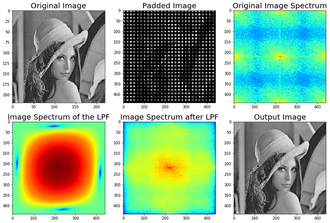
1. Using DFT to up-sample an image
- Let’s use the lena gray-scale image.
- First double the size of the by padding zero rows/columns at every alternate positions.
- Use FFT followed by an LPF.
- Finally use IFFT to get the output image.
The following code block shows the python code for implementing the steps listed above:
|
1
2
3
4
5
6
7
8
9
10
11
12
13
14
15
16
17
18
19
20
21
22
23
24
25
26
27
28
29
30
31
32
33
34
35
36
37
38
39
40
41
42
43
44
45
46
47
48
|
import numpy as npimport numpy.fft as fpimport matplotlib.pyplot as pltim = np.mean(imread('images/lena.jpg'), axis=2)im1 = np.zeros((2*im.shape[0], 2*im.shape[1]))print(im.shape, im1.shape)for i in range(im.shape[0]): for j in range(im.shape[1]): im1[2*i,2*j] = im[i,j]def padwithzeros(vector, pad_width, iaxis, kwargs): vector[:pad_width[0]] = 0 vector[-pad_width[1]:] = 0 return vector# the LPF kernelkernel = [[0.25, 0.5, 0.25], [0.5, 1, 0.5], [0.25, 0.5, 0.25]]# enlarge the kernel to the shape of the imagekernel = np.pad(kernel, (((im1.shape[0]-3)//2,(im1.shape[0]-3)//2+1), ((im1.shape[1]-3)//2,(im1.shape[1]-3)//2+1)), padwithzeros)plt.figure(figsize=(15,10))plt.gray() # show the filtered result in grayscalefreq = fp.fft2(im1)freq_kernel = fp.fft2(fp.ifftshift(kernel))freq_LPF = freq*freq_kernel # by the Convolution theoremim2 = fp.ifft2(freq_LPF)freq_im2 = fp.fft2(im2)plt.subplot(2,3,1)plt.imshow(im)plt.title('Original Image', size=20)plt.subplot(2,3,2)plt.imshow(im1)plt.title('Padded Image', size=20)plt.subplot(2,3,3)plt.imshow( (20*np.log10( 0.1 + fp.fftshift(freq))).astype(int), cmap='jet')plt.title('Original Image Spectrum', size=20)plt.subplot(2,3,4)plt.imshow( (20*np.log10( 0.1 + fp.fftshift(freq_kernel))).astype(int), cmap='jet')plt.title('Image Spectrum of the LPF', size=20)plt.subplot(2,3,5)plt.imshow( (20*np.log10( 0.1 + fp.fftshift(freq_im2))).astype(int), cmap='jet')plt.title('Image Spectrum after LPF', size=20)plt.subplot(2,3,6)plt.imshow(im2.astype(np.uint8)) # the imaginary part is an artifactplt.title('Output Image', size=20) |
The next figure shows the output. As can be seen from the next figure, the LPF removed the high frequency components from the Fourier spectrum of the padded image and with a subsequent inverse Fourier transform we get a decent enlarged image.
 https://sandipanweb.files.wordpress.com/2018/07/lena_lpf_fft.png?w=150 150w, https://sandipanweb.files.wordpress.com/2018/07/lena_lpf_fft.png?w=300 300w, https://sandipanweb.files.wordpress.com/2018/07/lena_lpf_fft.png?w=768 768w, https://sandipanweb.files.wordpress.com/2018/07/lena_lpf_fft.png 881w” sizes=”(max-width: 676px) 100vw, 676px” />
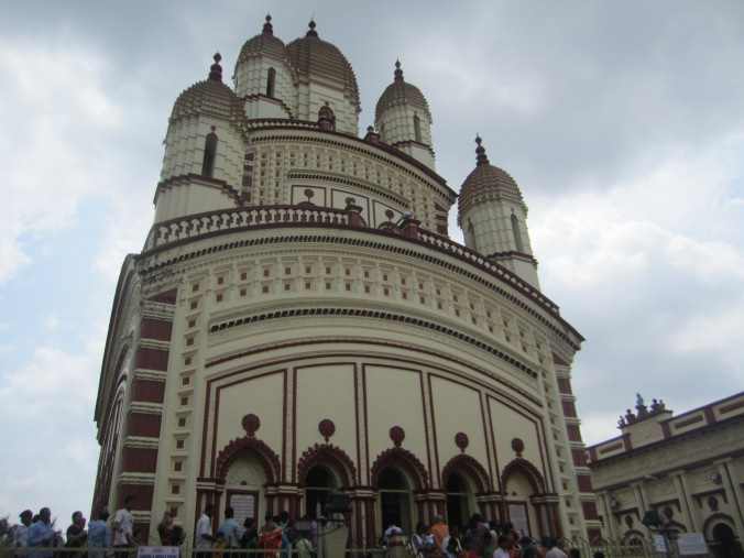
2. Frequency Domain Gaussian Filter
- Use an input image and use DFT to create the frequency 2D-array.
- Create a small Gaussian 2D Kernel (to be used as an LPF) in the spatial domain and pad it to enlarge it to the image dimensions.
- Use DFT to obtain the Gaussian Kernel in the frequency domain.
- Use the Convolution theorem to convolve the LPF with the input image in the frequency domain.
- Use IDFT to obtain the output image.
- Plot the frequency spectrum of the image, the gaussian kernel and the image obtained after convolution in the frequency domain, in 3D.
The following code block shows the python code:
|
1
2
3
4
5
6
7
8
9
10
11
12
13
14
15
16
17
18
19
20
21
22
23
24
25
26
27
|
import matplotlib.pyplot as pltfrom matplotlib import cmfrom skimage.color import rgb2grayfrom skimage.io import imreadimport scipy.fftpack as fpim = rgb2gray(imread('images/temple.jpg'))kernel = np.outer(signal.gaussian(im.shape[0], 10), signal.gaussian(im.shape[1], 10))freq = fp.fft2(im)assert(freq.shape == kernel.shape)freq_kernel = fp.fft2(fp.ifftshift(kernel))convolved = freq*freq_kernel # by the Convolution theoremim_blur = fp.ifft2(convolved).realim_blur = 255 * im_blur / np.max(im_blur)# center the frequency responseplt.imshow( (20*np.log10( 0.01 + fp.fftshift(freq_kernel))).real.astype(int), cmap='coolwarm')plt.colorbar()plt.show()plt.figure(figsize=(20,20))plt.imshow(im, cmap='gray')plt.show()from mpl_toolkits.mplot3d import Axes3Dfrom matplotlib.ticker import LinearLocator, FormatStrFormatter# ... code for 3D visualization of the spectrums |
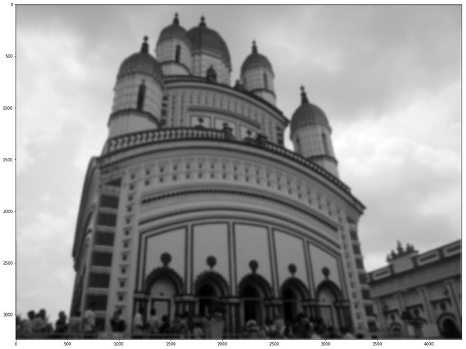
The original color temple image (time / spatial domain)
 https://sandipanweb.files.wordpress.com/2018/07/temple.jpg?w=1352 1352w, https://sandipanweb.files.wordpress.com/2018/07/temple.jpg?w=150 150w, https://sandipanweb.files.wordpress.com/2018/07/temple.jpg?w=300 300w, https://sandipanweb.files.wordpress.com/2018/07/temple.jpg?w=768 768w, https://sandipanweb.files.wordpress.com/2018/07/temple.jpg?w=1024 1024w” sizes=”(max-width: 676px) 100vw, 676px” />
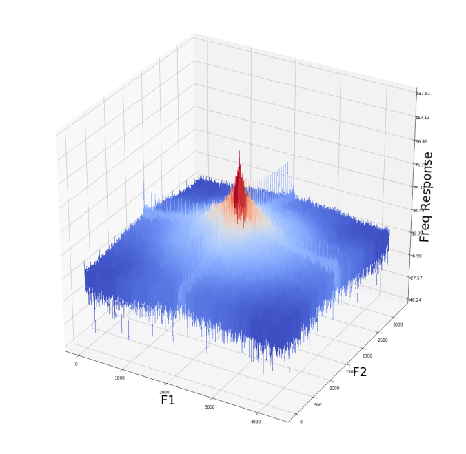
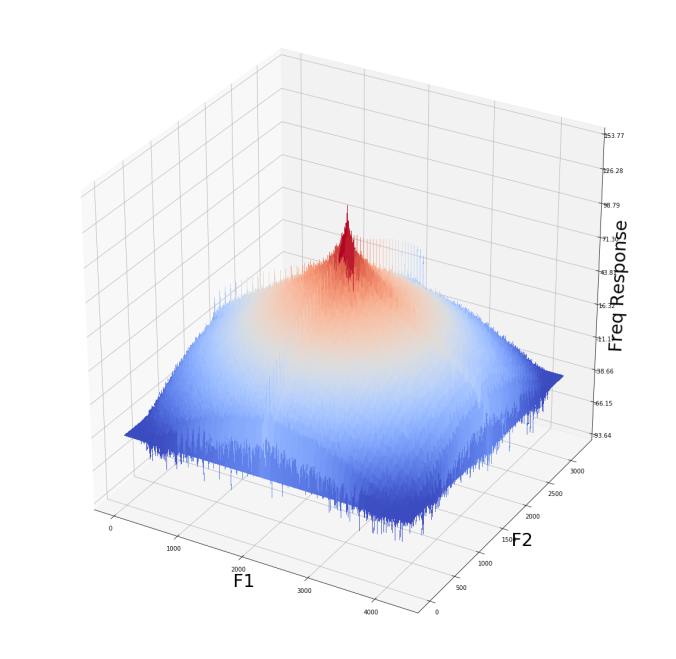
The temple image (frequency domain)
 https://sandipanweb.files.wordpress.com/2018/07/temple_freq.png?w=150 150w, https://sandipanweb.files.wordpress.com/2018/07/temple_freq.png?w=300 300w, https://sandipanweb.files.wordpress.com/2018/07/temple_freq.png?w=768 768w, https://sandipanweb.files.wordpress.com/2018/07/temple_freq.png?w=1024 1024w, https://sandipanweb.files.wordpress.com/2018/07/temple_freq.png 1137w” sizes=”(max-width: 676px) 100vw, 676px” />
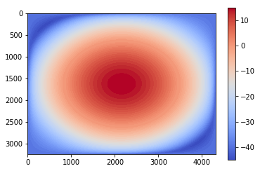
The Gaussian Kernel LPF in 2D (frequency domain)
 https://sandipanweb.files.wordpress.com/2018/07/gaussian_freq2d.png?w=150&h=99 150w, https://sandipanweb.files.wordpress.com/2018/07/gaussian_freq2d.png?w=300&h=198 300w” sizes=”(max-width: 801px) 100vw, 801px” />
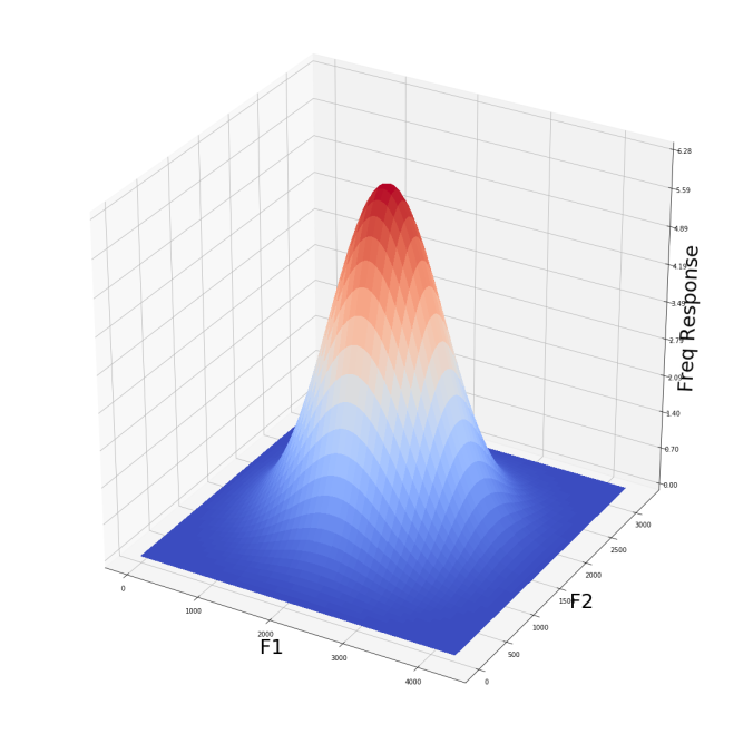
The Gaussian Kernel LPF (frequency domain)
 https://sandipanweb.files.wordpress.com/2018/07/gaussian_freq.png?w=150 150w, https://sandipanweb.files.wordpress.com/2018/07/gaussian_freq.png?w=300 300w, https://sandipanweb.files.wordpress.com/2018/07/gaussian_freq.png?w=768 768w, https://sandipanweb.files.wordpress.com/2018/07/gaussian_freq.png?w=1024 1024w, https://sandipanweb.files.wordpress.com/2018/07/gaussian_freq.png 1137w” sizes=”(max-width: 676px) 100vw, 676px” />
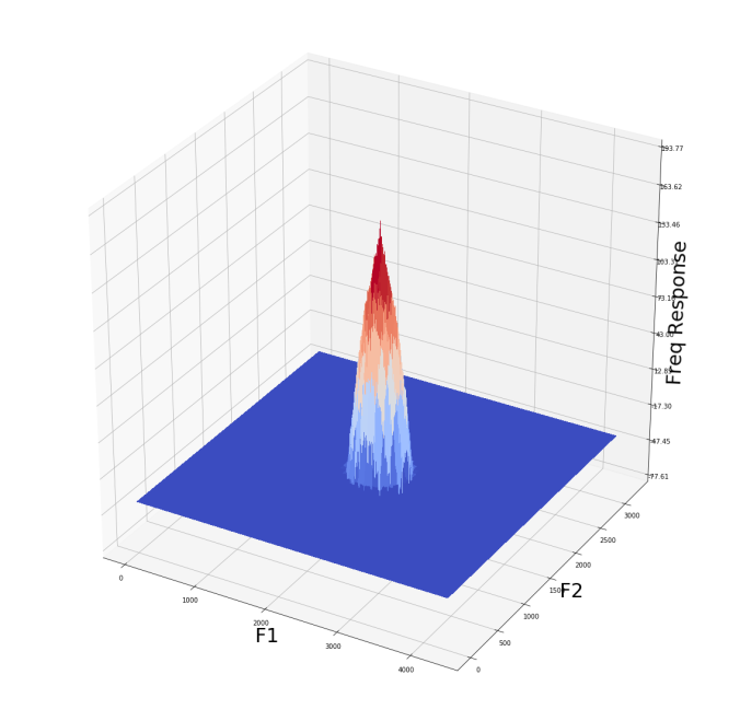
The smoothed temple image with the LPF (frequency domain)
 https://sandipanweb.files.wordpress.com/2018/07/temple_freq_lpf.png?w=150 150w, https://sandipanweb.files.wordpress.com/2018/07/temple_freq_lpf.png?w=300 300w, https://sandipanweb.files.wordpress.com/2018/07/temple_freq_lpf.png?w=768 768w, https://sandipanweb.files.wordpress.com/2018/07/temple_freq_lpf.png?w=1024 1024w, https://sandipanweb.files.wordpress.com/2018/07/temple_freq_lpf.png 1137w” sizes=”(max-width: 676px) 100vw, 676px” />
If we set the standard deviation of the LPF Gaussian kernel to be 10 we get the following output as shown in the next figures. As can be seen, the frequency response value drops much quicker from the center.
The smoothed temple image with the LPF with higher s.d. (frequency domain)
 https://sandipanweb.files.wordpress.com/2018/07/temple_freq_lpf2.png?w=150 150w, https://sandipanweb.files.wordpress.com/2018/07/temple_freq_lpf2.png?w=300 300w, https://sandipanweb.files.wordpress.com/2018/07/temple_freq_lpf2.png?w=768 768w, https://sandipanweb.files.wordpress.com/2018/07/temple_freq_lpf2.png?w=1024 1024w, https://sandipanweb.files.wordpress.com/2018/07/temple_freq_lpf2.png 1137w” sizes=”(max-width: 676px) 100vw, 676px” />
The output image after convolution (spatial / time domain)
 https://sandipanweb.files.wordpress.com/2018/07/temple_blurred.png?w=150 150w, https://sandipanweb.files.wordpress.com/2018/07/temple_blurred.png?w=300 300w, https://sandipanweb.files.wordpress.com/2018/07/temple_blurred.png?w=768 768w, https://sandipanweb.files.wordpress.com/2018/07/temple_blurred.png?w=1024 1024w, https://sandipanweb.files.wordpress.com/2018/07/temple_blurred.png 1166w” sizes=”(max-width: 676px) 100vw, 676px” />
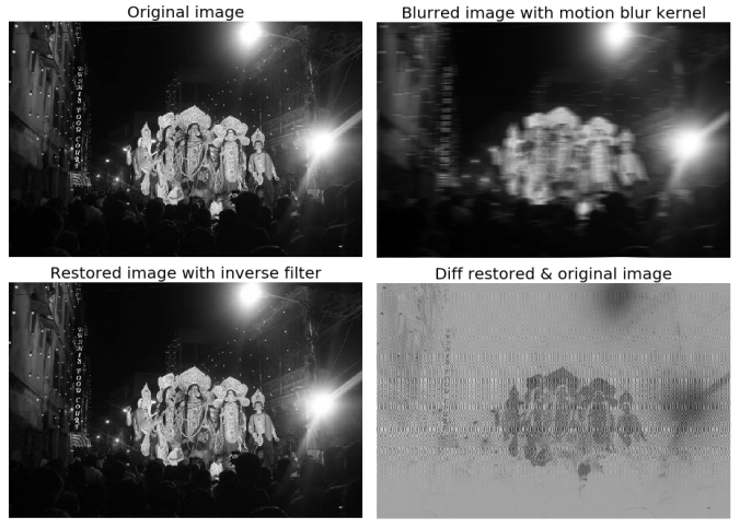
3. Using the inverse filter to restore a motion-blurred image
- First create a motion blur kernel of a given shape.
- Convolve the kernel with an input image in the frequency domain.
- Get the motion-blurred image in the spatial domain with IDFT.
- Compute the inverse filter kernel and convolve with the blurred image in the frequency domain.
- Get the convolved image back in the spatial domain.
- Plot all the images and kernels in the frequency domain.
The following code block shows the python code:
|
1
2
3
4
5
6
7
8
9
10
11
12
13
14
15
16
17
18
19
20
21
22
23
24
25
26
27
28
29
30
31
32
33
34
35
36
37
38
39
40
41
42
43
|
im = rgb2gray(imread('../my images/madurga.jpg'))# create the motion blur kernelsize = 21kernel = np.zeros((size, size))kernel[int((size-1)/2), :] = np.ones(size)kernel = kernel / sizekernel = np.pad(kernel, (((im.shape[0]-size)//2,(im.shape[0]-size)//2+1), ((im.shape[1]-size)//2,(im.shape[1]-size)//2+1)), padwithzeros)freq = fp.fft2(im)freq_kernel = fp.fft2(fp.ifftshift(kernel))convolved1 = freq1*freq_kernel1im_blur = fp.ifft2(convolved1).realim_blur = im_blur / np.max(im_blur)epsilon = 10**-6freq = fp.fft2(im_blur)freq_kernel = 1 / (epsilon + freq_kernel1)convolved = freq*freq_kernelim_restored = fp.ifft2(convolved).realim_restored = im_restored / np.max(im_restored)plt.figure(figsize=(18,12))plt.subplot(221)plt.imshow(im)plt.title('Original image', size=20)plt.axis('off')plt.subplot(222)plt.imshow(im_blur)plt.title('Blurred image with motion blur kernel', size=20)plt.axis('off')plt.subplot(223)plt.imshow(im_restored)plt.title('Restored image with inverse filter', size=20)plt.axis('off')plt.subplot(224)plt.imshow(im_restored - im)plt.title('Diff restored & original image', size=20)plt.axis('off')plt.show()# Plot the surface of the frequency responses here |
 https://sandipanweb.files.wordpress.com/2018/07/madurga_inverse.png?w=150 150w, https://sandipanweb.files.wordpress.com/2018/07/madurga_inverse.png?w=300 300w, https://sandipanweb.files.wordpress.com/2018/07/madurga_inverse.png?w=768 768w, https://sandipanweb.files.wordpress.com/2018/07/madurga_inverse.png 931w” sizes=”(max-width: 676px) 100vw, 676px” />
Frequency response of the input image
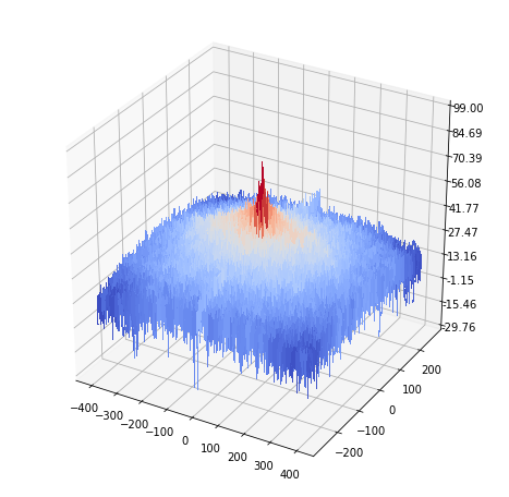 https://sandipanweb.files.wordpress.com/2018/07/madurga_freq.png?w=150&h=146 150w, https://sandipanweb.files.wordpress.com/2018/07/madurga_freq.png?w=300&h=293 300w” sizes=”(max-width: 630px) 100vw, 630px” />
(log) Frequency response of the motion blur kernel (LPF)
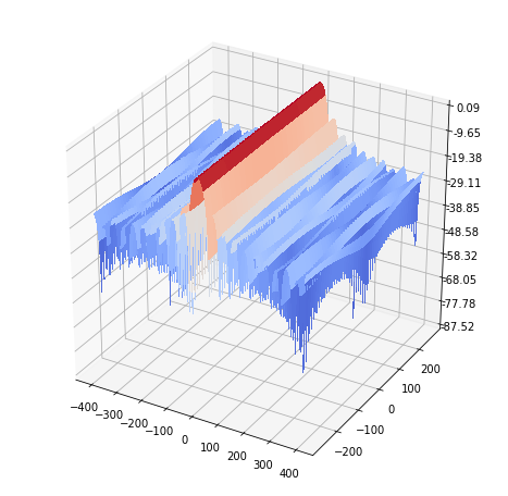 https://sandipanweb.files.wordpress.com/2018/07/motion_blur_freq1.png?w=150&h=146 150w, https://sandipanweb.files.wordpress.com/2018/07/motion_blur_freq1.png?w=300&h=293 300w” sizes=”(max-width: 693px) 100vw, 693px” />
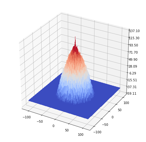
Input image convolved with the motion blur kernel (frequency domain)
 https://sandipanweb.files.wordpress.com/2018/07/madurga_convolved11.png?w=150&h=146 150w, https://sandipanweb.files.wordpress.com/2018/07/madurga_convolved11.png?w=300&h=293 300w” sizes=”(max-width: 637px) 100vw, 637px” />
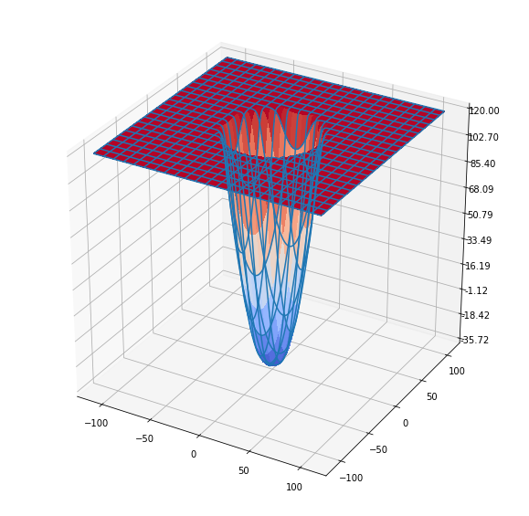
(log) Frequency response of the inverse frequency filter kernel (HPF)
 https://sandipanweb.files.wordpress.com/2018/07/motion_blur_freq.png?w=150&h=146 150w, https://sandipanweb.files.wordpress.com/2018/07/motion_blur_freq.png?w=300&h=293 300w” sizes=”(max-width: 636px) 100vw, 636px” />
Motion-blurred image convolved with the inverse frequency filter kernel (frequency domain)
 https://sandipanweb.files.wordpress.com/2018/07/madurga_convolved.png?w=150 150w, https://sandipanweb.files.wordpress.com/2018/07/madurga_convolved.png?w=300 300w” sizes=”(max-width: 583px) 100vw, 583px” />
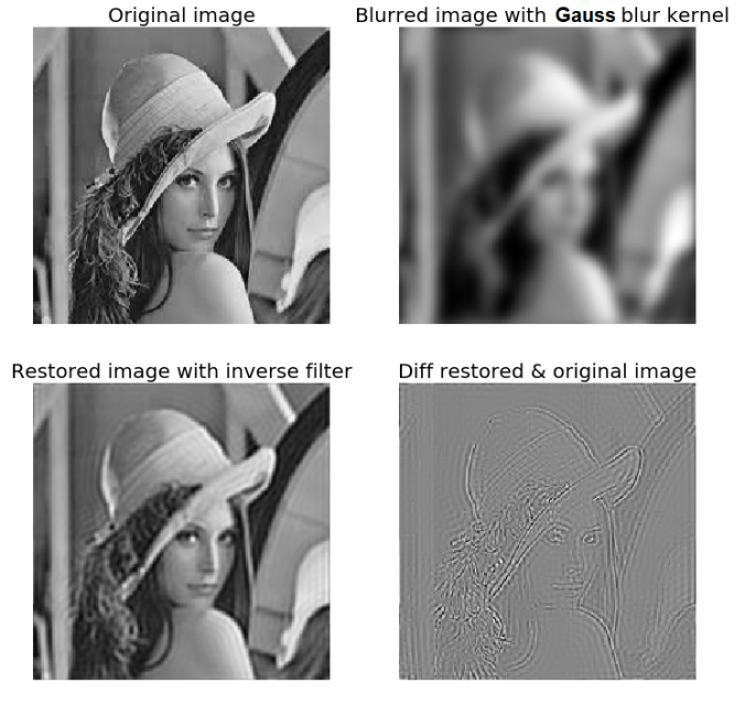
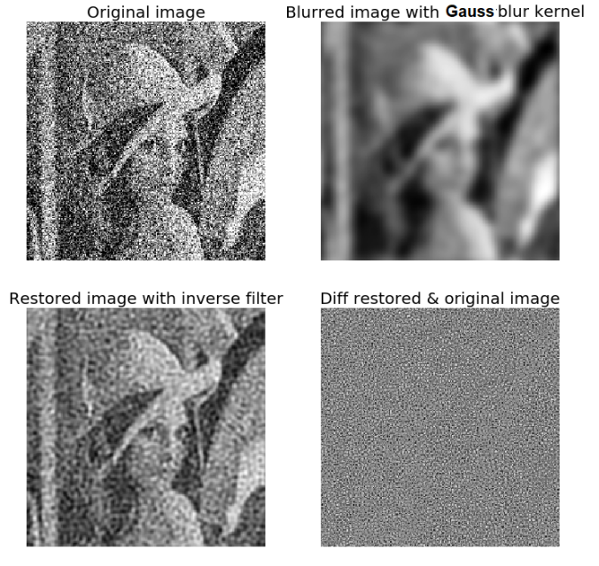
4. Impact of noise on the inverse filter
- Add some random noise to the Lena image.
- Blur the image with a Gaussian kernel.
- Restore the image using inverse filter.
With the original image
Let’s first blur and apply the inverse filter on the noiseless blurred image. The following figures show the outputs:
 https://sandipanweb.files.wordpress.com/2018/07/lena_inverse.png?w=150 150w, https://sandipanweb.files.wordpress.com/2018/07/lena_inverse.png?w=300 300w, https://sandipanweb.files.wordpress.com/2018/07/lena_inverse.png 745w” sizes=”(max-width: 676px) 100vw, 676px” />
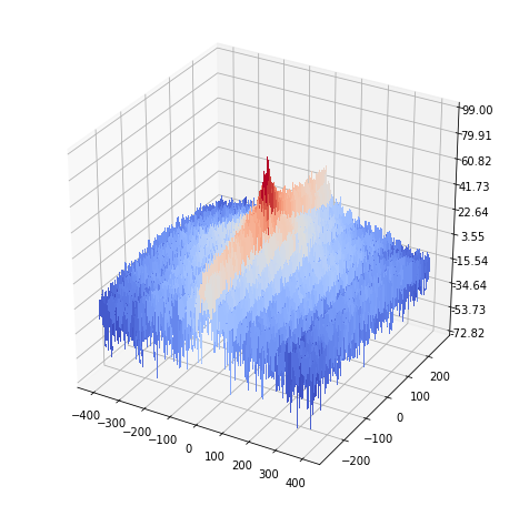
(log) Frequency response of the input image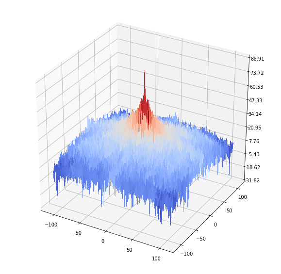 https://sandipanweb.files.wordpress.com/2018/07/lena_freq.png?w=150 150w, https://sandipanweb.files.wordpress.com/2018/07/lena_freq.png?w=300 300w” sizes=”(max-width: 579px) 100vw, 579px” />
(log) Frequency response of the Gaussian blur kernel (LPF)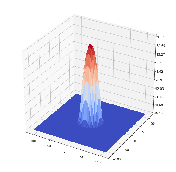 https://sandipanweb.files.wordpress.com/2018/07/lena_gaussian_freq.png?w=150&h=146 150w, https://sandipanweb.files.wordpress.com/2018/07/lena_gaussian_freq.png?w=300&h=293 300w” sizes=”(max-width: 635px) 100vw, 635px” />
(log) Frequency response of the blurred image
 https://sandipanweb.files.wordpress.com/2018/07/lena_blurred_spectrum.png?w=150&h=146 150w, https://sandipanweb.files.wordpress.com/2018/07/lena_blurred_spectrum.png?w=300&h=293 300w” sizes=”(max-width: 621px) 100vw, 621px” />
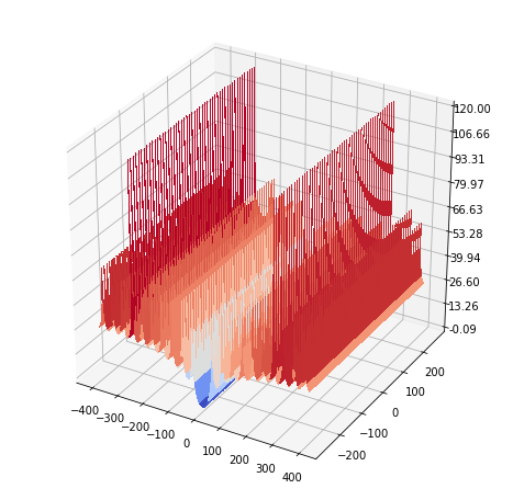
(log) Frequency response of the inverse kernel (HPF)
 https://sandipanweb.files.wordpress.com/2018/07/gauss_inverse_kernel.png?w=150 150w, https://sandipanweb.files.wordpress.com/2018/07/gauss_inverse_kernel.png?w=300 300w” sizes=”(max-width: 639px) 100vw, 639px” />
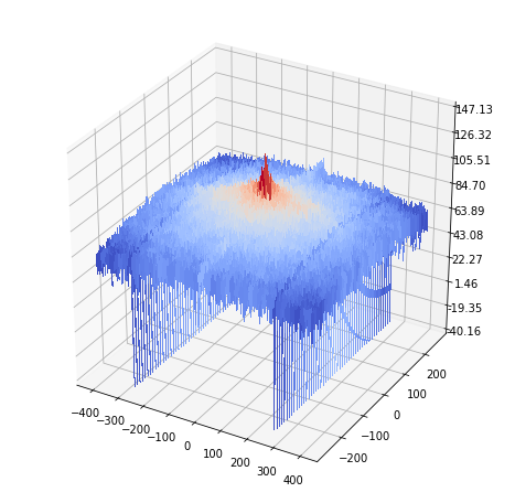
Frequency response of the output image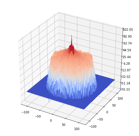 https://sandipanweb.files.wordpress.com/2018/07/lena_inverse_spectrum.png?w=150&h=146 150w, https://sandipanweb.files.wordpress.com/2018/07/lena_inverse_spectrum.png?w=300&h=293 300w” sizes=”(max-width: 563px) 100vw, 563px” />
Adding noise to the original image
The following python code can be used to add Gaussian noise to an image:
|
1
2
|
from skimage.util import random_noiseim = random_noise(im, var=0.1) |
The next figures show the noisy lena image, the blurred image with a Gaussian Kernel and the restored image with the inverse filter. As can be seen, being a high-pass filter, the inverse filter enhances the noise, typically corresponding to high frequencies.
 https://sandipanweb.files.wordpress.com/2018/07/lena_noisy_inverse1.png?w=150 150w, https://sandipanweb.files.wordpress.com/2018/07/lena_noisy_inverse1.png?w=300 300w, https://sandipanweb.files.wordpress.com/2018/07/lena_noisy_inverse1.png 745w” sizes=”(max-width: 676px) 100vw, 676px” />
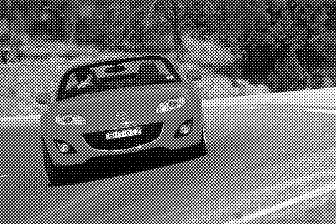
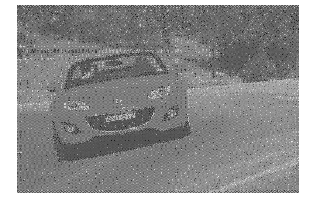
5. Use a notch filter to remove periodic noise from the following half-toned car image.
 https://sandipanweb.files.wordpress.com/2018/07/halftone.png?w=150 150w, https://sandipanweb.files.wordpress.com/2018/07/halftone.png?w=300 300w, https://sandipanweb.files.wordpress.com/2018/07/halftone.png?w=768 768w, https://sandipanweb.files.wordpress.com/2018/07/halftone.png 1000w” sizes=”(max-width: 676px) 100vw, 676px” />
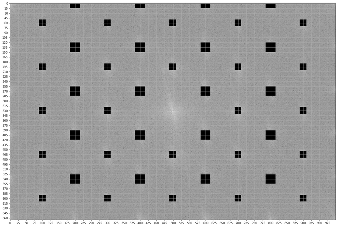
- Use DFT to obtain the frequency spectrum of the image.
- Block the high frequency components that are most likely responsible fro noise.
- Use IDFT to come back to the spatial domain.
|
1
2
3
4
5
6
7
8
9
10
11
12
13
14
15
16
17
18
19
20
|
from scipy import fftpackim = imread('images/halftone.png')F1 = fftpack.fft2((im).astype(float))F2 = fftpack.fftshift(F1)for i in range(60, w, 135):for j in range(100, h, 200):if not (i == 330 and j == 500):F2[i-10:i+10, j-10:j+10] = 0for i in range(0, w, 135):for j in range(200, h, 200):if not (i == 330 and j == 500):F2[max(0,i-15):min(w,i+15), max(0,j-15):min(h,j+15)] = 0plt.figure(figsize=(6.66,10))plt.imshow( (20*np.log10( 0.1 + F2)).astype(int), cmap=plt.cm.gray)plt.show()im1 = fp.ifft2(fftpack.ifftshift(F2)).realplt.figure(figsize=(10,10))plt.imshow(im1, cmap='gray')plt.axis('off')plt.show() |
Frequency response of the input image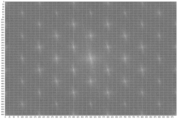 https://sandipanweb.files.wordpress.com/2018/07/car_freq.png?w=150 150w, https://sandipanweb.files.wordpress.com/2018/07/car_freq.png?w=300 300w, https://sandipanweb.files.wordpress.com/2018/07/car_freq.png?w=768 768w, https://sandipanweb.files.wordpress.com/2018/07/car_freq.png?w=1024 1024w, https://sandipanweb.files.wordpress.com/2018/07/car_freq.png 1160w” sizes=”(max-width: 676px) 100vw, 676px” />
Frequency response of the input image with blocked frequencies with notch
 https://sandipanweb.files.wordpress.com/2018/07/car_notch_blocked.png?w=150 150w, https://sandipanweb.files.wordpress.com/2018/07/car_notch_blocked.png?w=300 300w, https://sandipanweb.files.wordpress.com/2018/07/car_notch_blocked.png?w=768 768w, https://sandipanweb.files.wordpress.com/2018/07/car_notch_blocked.png?w=1024 1024w, https://sandipanweb.files.wordpress.com/2018/07/car_notch_blocked.png 1160w” sizes=”(max-width: 676px) 100vw, 676px” />
Output image
 https://sandipanweb.files.wordpress.com/2018/07/car_notch1.png?w=150&h=100 150w, https://sandipanweb.files.wordpress.com/2018/07/car_notch1.png?w=300&h=199 300w” sizes=”(max-width: 718px) 100vw, 718px” />
With a low-pass-filter (LPF):
Frequency response of the input image with blocked frequencies with LPF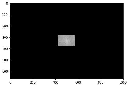 https://sandipanweb.files.wordpress.com/2018/07/car_freq_notch.png?w=150&h=100 150w, https://sandipanweb.files.wordpress.com/2018/07/car_freq_notch.png?w=300&h=200 300w” sizes=”(max-width: 696px) 100vw, 696px” />
Output image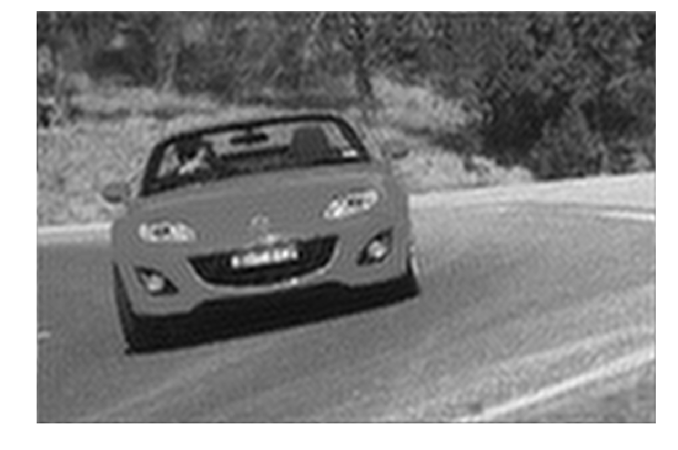 https://sandipanweb.files.wordpress.com/2018/07/car_notch.png?w=150&h=100 150w, https://sandipanweb.files.wordpress.com/2018/07/car_notch.png?w=300&h=199 300w” sizes=”(max-width: 775px) 100vw, 775px” />