Solving Some Image Processing Problems with Python libraries - Part 3

Uncategorized

Solving Some Image Processing Problems with Python libraries – Part 3

MMS • RSS

Article originally posted on Data Science Central. Visit Data Science Central

In this article a few more popular image processing problems along with their solutions are going to be discussed. Python image processing libraries are going to be used to solve these problems.

Histogram Matching with color images

As described here, here is the algorithm:

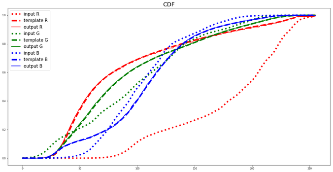
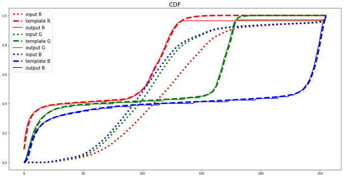
The cumulative histogram is computed for each image dataset, see the figure below.
For any particular value (x_i) in the input image data to be adjusted has a cumulative histogram value given by G(x_i).
This in turn is the cumulative distribution value in the reference (template) image dataset, namely H(x_j). The input data value x_i is replaced by x_j.

im = imread('images/lena.jpg')
im_t = imread('my images/vstyle.png')
im1 = np.zeros(im.shape).astype(np.uint8)
plt.figure(figsize=(20,10))
for i in range(3):
    c = cdf(im[...,i])
    c_t = cdf(im_t[...,i])
    im1[...,i] = hist_matching(c, c_t, im[...,i]) # implement this function with the above algorithm
    c1 = cdf(im1[...,i])
    col = 'r' if i == 0 else ('g' if i == 1 else 'b')
    plt.plot(np.arange(256), c, col + ':', label='input ' + col.upper(), linewidth=5)
    plt.plot(np.arange(256), c_t, col + '--', label='template ' + col.upper(), linewidth=5)
    plt.plot(np.arange(256), c1, col + '-', label='output ' + col.upper(), linewidth=2)
plt.title('CDF', size=20)
plt.legend(prop={'size': 15})
plt.show()
 
plt.figure(figsize=(10,10))
plt.imshow(im1[...,:3])
plt.axis('off')
plt.show()

Input image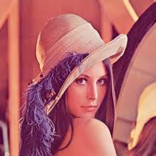
lena https://sandipanweb.files.wordpress.com/2018/07/lena1.jpg?w=150&h=150 150w” sizes=”(max-width: 401px) 100vw, 401px” />

Template Image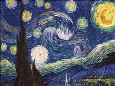 vstyle https://sandipanweb.files.wordpress.com/2018/07/vstyle.png?w=150&h=113 150w, https://sandipanweb.files.wordpress.com/2018/07/vstyle.png?w=300&h=225 300w” sizes=”(max-width: 571px) 100vw, 571px” />

Output Image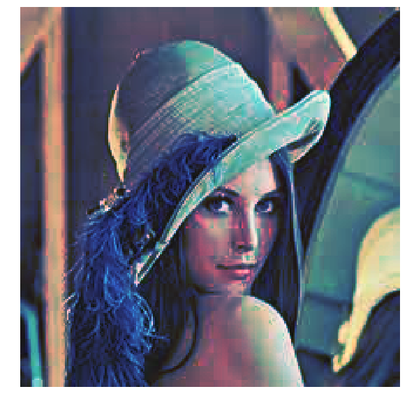
https://sandipanweb.files.wordpress.com/2018/07/lena_starry.png?w=150 150w, https://sandipanweb.files.wordpress.com/2018/07/lena_starry.png?w=300 300w” sizes=”(max-width: 583px) 100vw, 583px” />

The following figure shows how the histogram of the input image is matched with the histogram of the template image.

https://sandipanweb.files.wordpress.com/2018/07/lena_starry_cdf.png?w=150 150w, https://sandipanweb.files.wordpress.com/2018/07/lena_starry_cdf.png?w=300 300w, https://sandipanweb.files.wordpress.com/2018/07/lena_starry_cdf.png?w=768 768w, https://sandipanweb.files.wordpress.com/2018/07/lena_starry_cdf.png?w=1024 1024w, https://sandipanweb.files.wordpress.com/2018/07/lena_starry_cdf.png 1153w” sizes=”(max-width: 676px) 100vw, 676px” />

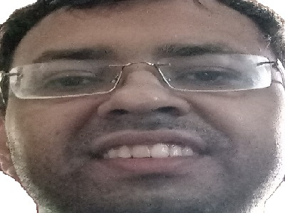
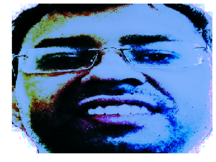
Another example:

Input image

me1 https://sandipanweb.files.wordpress.com/2018/07/me1.jpg?w=150 150w, https://sandipanweb.files.wordpress.com/2018/07/me1.jpg?w=300 300w” sizes=”(max-width: 400px) 100vw, 400px” />

Template Image

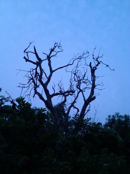https://sandipanweb.files.wordpress.com/2018/07/treebirds.jpg?w=113 113w, https://sandipanweb.files.wordpress.com/2018/07/treebirds.jpg?w=225 225w” sizes=”(max-width: 450px) 100vw, 450px” />

Output Image

me_t https://sandipanweb.files.wordpress.com/2018/07/me_t.png?w=150&h=113 150w, https://sandipanweb.files.wordpress.com/2018/07/me_t.png?w=300&h=226 300w, https://sandipanweb.files.wordpress.com/2018/07/me_t.png 601w” sizes=”(max-width: 421px) 100vw, 421px” />

me_hm https://sandipanweb.files.wordpress.com/2018/07/me_hm.png?w=150 150w, https://sandipanweb.files.wordpress.com/2018/07/me_hm.png?w=300 300w, https://sandipanweb.files.wordpress.com/2018/07/me_hm.png?w=768 768w, https://sandipanweb.files.wordpress.com/2018/07/me_hm.png?w=1024 1024w, https://sandipanweb.files.wordpress.com/2018/07/me_hm.png 1156w” sizes=”(max-width: 676px) 100vw, 676px” />

Mathematical Morphology

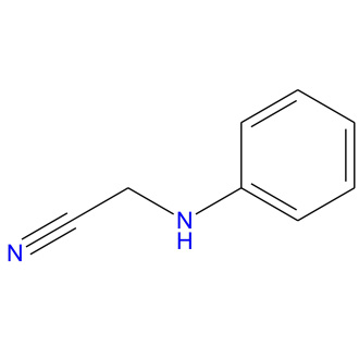
1. Automatically cropping an image

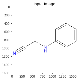
Let’s use the following image. The image has unnecessary white background outside the molecule of the organic compound.https://sandipanweb.files.wordpress.com/2018/07/l_2d.jpg?w=660&h=660 660w, https://sandipanweb.files.wordpress.com/2018/07/l_2d.jpg?w=150&h=150 150w, https://sandipanweb.files.wordpress.com/2018/07/l_2d.jpg?w=300&h=300 300w” sizes=”(max-width: 330px) 100vw, 330px” />
First convert the image to a binary image and compute the convex hull of the molecule object.
Use the convex hull image to find the bounding box for cropping.
Crop the original image with the bounding box.

The next python code shows how to implement the above steps:

from PIL import Image
from skimage.io import imread
from skimage.morphology import convex_hull_image
im = imread('../images/L_2d.jpg')
plt.imshow(im)
plt.title('input image')
plt.show()
im1 = 1 - rgb2gray(im)
threshold = 0.5
im1[im1  threshold] = 1
chull = convex_hull_image(im1)
plt.imshow(chull)
plt.title('convex hull in the binary image')
plt.show()
imageBox = Image.fromarray((chull*255).astype(np.uint8)).getbbox()
cropped = Image.fromarray(im).crop(imageBox)
cropped.save('L_2d_cropped.jpg')
plt.imshow(cropped)
plt.title('cropped image')
plt.show()&amp;amp;amp;amp;amp;amp;amp;amp;amp;amp;amp;amp;nbsp; &amp;amp;amp;amp;amp;amp;amp;amp;amp;amp;amp;amp;nbsp; &amp;amp;amp;amp;amp;amp;amp;amp;amp;amp;amp;amp;nbsp;

chem1 https://sandipanweb.files.wordpress.com/2018/07/chem11.png?w=150&h=148 150w” sizes=”(max-width: 339px) 100vw, 339px” /> 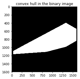chem2 https://sandipanweb.files.wordpress.com/2018/07/chem2.png?w=150&h=148 150w” sizes=”(max-width: 340px) 100vw, 340px” /> 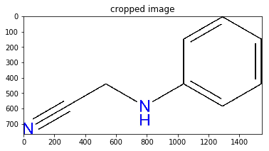chem3 https://sandipanweb.files.wordpress.com/2018/07/chem3.png?w=150 150w, https://sandipanweb.files.wordpress.com/2018/07/chem3.png?w=300 300w” sizes=”(max-width: 378px) 100vw, 378px” />

This can also be found here.

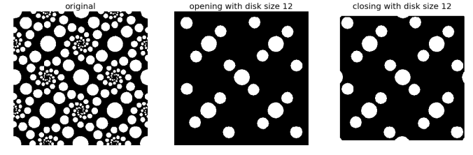
2. Opening and Closing are Dual operations in mathematical morphology

Start with a binary image and apply opening operation with some structuring element (e.g., a disk) on it to obtain an output image.
Invert the image (to change the foreground to background and vice versa) and apply closing operation on it with the same structuring element to obtain another output image.
Invert the second output image obtained and observe that it’s same as the first output image.
Thus applying opening operation to the foreground of a binary image is equivalent to applying closing operation to the background of the same image with the same structuring element.

The next python code shows the implementation of the above steps.

from skimage.morphology import binary_opening, binary_closing, disk
from skimage.util import invert
im = rgb2gray(imread('../new images/circles.jpg'))
im[im  0.5] = 1
plt.gray()
plt.figure(figsize=(20,10))
plt.subplot(131)
plt.imshow(im)
plt.title('original', size=20)
plt.axis('off')
plt.subplot(1,3,2)
im1 = binary_opening(im, disk(12))
plt.imshow(im1)
plt.title('opening with disk size ' + str(12), size=20)
plt.axis('off')
plt.subplot(1,3,3)
im1 = invert(binary_closing(invert(im), disk(12)))
plt.imshow(im1)
plt.title('closing with disk size ' + str(12), size=20)
plt.axis('off')
plt.show()

As can be seen the output images obtained are exactly same.

https://sandipanweb.files.wordpress.com/2018/07/opening_closing_dual.png?w=150 150w, https://sandipanweb.files.wordpress.com/2018/07/opening_closing_dual.png?w=300 300w, https://sandipanweb.files.wordpress.com/2018/07/opening_closing_dual.png?w=768 768w, https://sandipanweb.files.wordpress.com/2018/07/opening_closing_dual.png?w=1024 1024w, https://sandipanweb.files.wordpress.com/2018/07/opening_closing_dual.png 1159w” sizes=”(max-width: 676px) 100vw, 676px” />

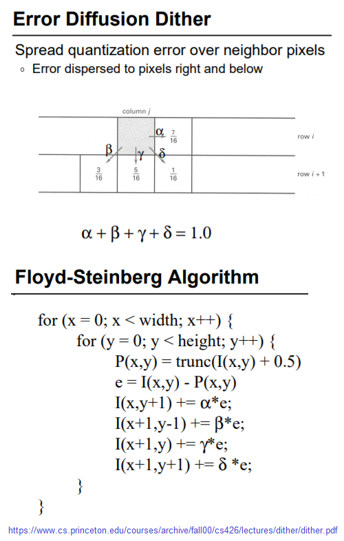
Floyd-Steinberg Dithering (to convert a grayscale to a binary image)

The next figure shows the algorithm for error diffusion dithering.

https://sandipanweb.files.wordpress.com/2018/07/fsa.png?w=95 95w, https://sandipanweb.files.wordpress.com/2018/07/fsa.png?w=191 191w” sizes=”(max-width: 500px) 100vw, 500px” />

def find_closest_palette_color(oldpixel):
    return int(round(oldpixel / 255)*255)
 
im = rgb2gray(imread('../my images/godess.jpg'))*255
pixel = np.copy(im)
w, h = im.shape
 
for x in range(w):
    for y in range(h):
        oldpixel = pixel[x][y]
        newpixel = find_closest_palette_color(oldpixel)
        pixel[x][y] = newpixel
        quant_error = oldpixel - newpixel
        if x + 1 &amp;amp;amp;amp;amp;amp;amp;amp;amp;amp;amp;amp;lt; w-1:
          pixel[x + 1][y] = pixel[x + 1][y] + quant_error * 7 / 16
        if x &amp;amp;amp;amp;amp;amp;amp;amp;amp;amp;amp;amp;gt; 0 and y &amp;amp;amp;amp;amp;amp;amp;amp;amp;amp;amp;amp;lt; h-1:
           pixel[x - 1][y + 1] = pixel[x - 1][y + 1] + quant_error * 3 / 16
        if y &amp;amp;amp;amp;amp;amp;amp;amp;amp;amp;amp;amp;lt; h-1:
           pixel[x ][y + 1] = pixel[x ][y + 1] + quant_error * 5 / 16
        if x &amp;amp;amp;amp;amp;amp;amp;amp;amp;amp;amp;amp;lt; w-1 and y &amp;amp;amp;amp;amp;amp;amp;amp;amp;amp;amp;amp;lt; h-1:
           pixel[x + 1][y + 1] = pixel[x + 1][y + 1] + quant_error * 1 / 16
 
plt.figure(figsize=(10,20))
plt.imshow(pixel, cmap='gray')
plt.axis('off')
plt.show()

The input image (gray-scale)

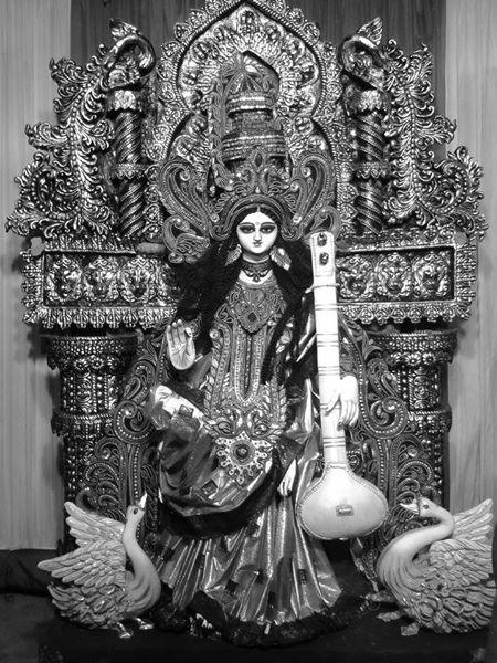https://sandipanweb.files.wordpress.com/2018/07/godess_gray.jpg?w=113&h=150 113w, https://sandipanweb.files.wordpress.com/2018/07/godess_gray.jpg?w=225&h=300 225w” sizes=”(max-width: 557px) 100vw, 557px” />

The output Image (binary)

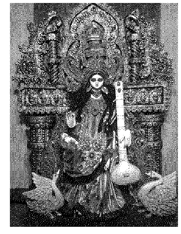https://sandipanweb.files.wordpress.com/2018/07/godess_binary.png?w=116 116w, https://sandipanweb.files.wordpress.com/2018/07/godess_binary.png?w=232 232w” sizes=”(max-width: 601px) 100vw, 601px” />

The next animation shows how an another input grayscale image gets converted to output binary image using the error diffusion dithering.

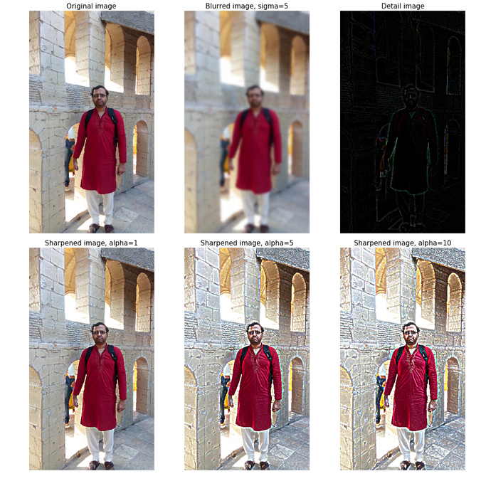
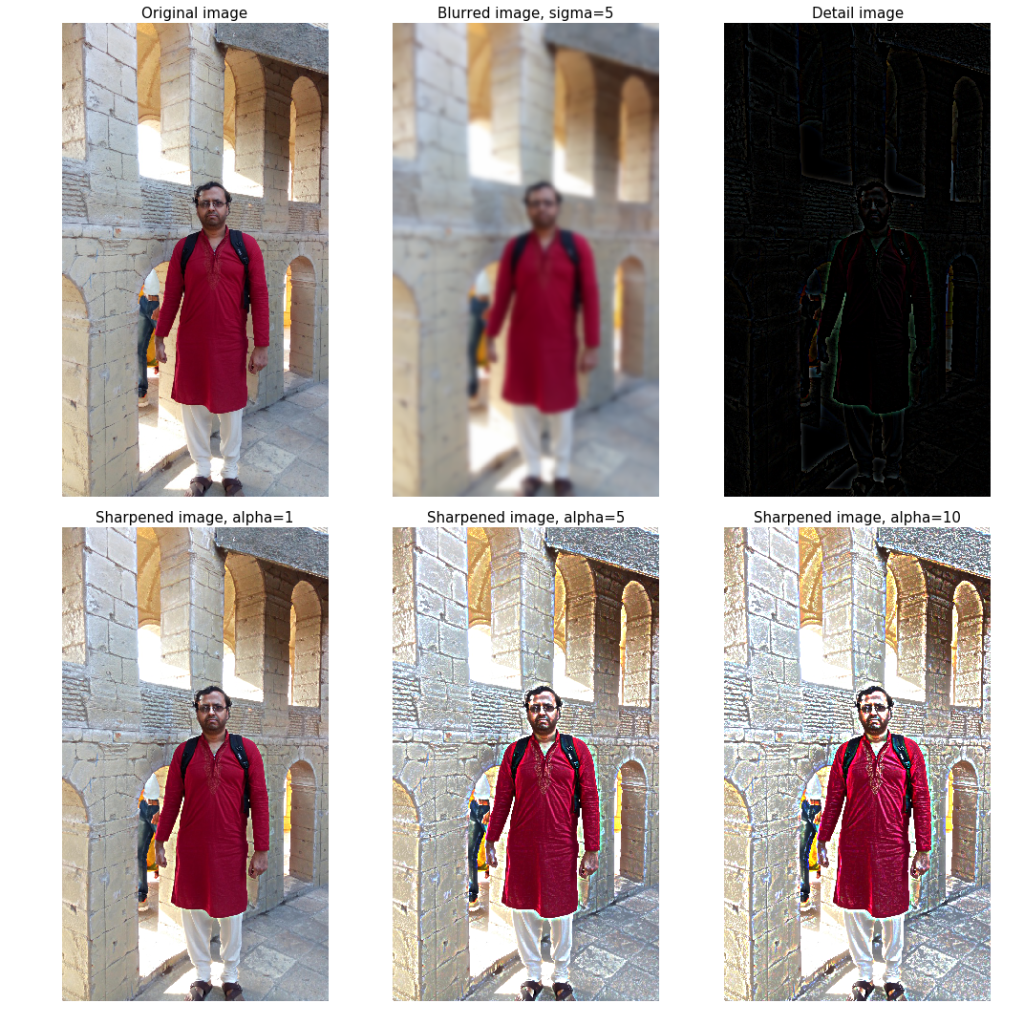
Sharpen a color image

First blur the image with an LPF (e.g., Gaussian Filter).
Compute the detail image as the difference between the original and the blurred image.
Now the sharpened image can be computed as a linear combination of the original image and the detail image. The next figure illustrates the concept.

https://sandipanweb.files.wordpress.com/2018/07/f8.png?w=150 150w, https://sandipanweb.files.wordpress.com/2018/07/f8.png?w=300 300w, https://sandipanweb.files.wordpress.com/2018/07/f8.png 742w” sizes=”(max-width: 676px) 100vw, 676px” />

The next python code shows how this can be implemented in python:

from scipy import misc, ndimage
import matplotlib.pyplot as plt
import numpy as np
 
def rgb2gray(im):
    return np.clip(0.2989 * im[...,0] + 0.5870 * im[...,1] + 0.1140 * im[...,2], 0, 1)
 
im = misc.imread('../my images/me.jpg')/255
im_blurred = ndimage.gaussian_filter(im, (5,5,0))
im_detail = np.clip(im - im_blurred, 0, 1)
fig, axes = plt.subplots(nrows=2, ncols=3, sharex=True, sharey=True, figsize=(15, 15))
axes = axes.ravel()
axes[0].imshow(im)
axes[0].set_title('Original image', size=15)
axes[1].imshow(im_blurred)
axes[1].set_title('Blurred image, sigma=5', size=15)
axes[2].imshow(im_detail)
axes[2].set_title('Detail image', size=15)
alpha = [1, 5, 10]
for i in range(3):
    im_sharp = np.clip(im + alpha[i]*im_detail, 0, 1)
    axes[3+i].imshow(im_sharp)
    axes[3+i].set_title('Sharpened image, alpha=' + str(alpha[i]), size=15)
for ax in axes:
    ax.axis('off')
fig.tight_layout()
plt.show()

The next figure shows the output of the above code block. As cane be seen, the output gets more sharpened as the value of alpha gets increased.

https://sandipanweb.files.wordpress.com/2018/07/me_unsharp2.png?w=150 150w, https://sandipanweb.files.wordpress.com/2018/07/me_unsharp2.png?w=300 300w, https://sandipanweb.files.wordpress.com/2018/07/me_unsharp2.png?w=768 768w, https://sandipanweb.files.wordpress.com/2018/07/me_unsharp2.png?w=1024 1024w, https://sandipanweb.files.wordpress.com/2018/07/me_unsharp2.png 1072w” sizes=”(max-width: 676px) 100vw, 676px” />

The next animation shows how the image gets more and more sharpened with increasing alpha.

me_sharp

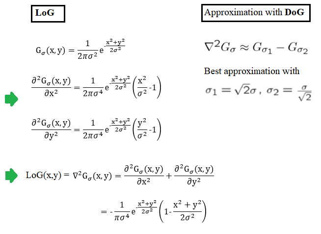
Edge Detection with LOG and Zero-Crossing Algorithm by Marr and Hildreth

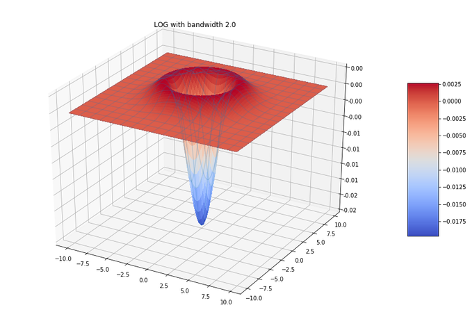
The following figure shows LOG filter and its DOG approximation.

https://sandipanweb.files.wordpress.com/2018/07/f1.png?w=150 150w, https://sandipanweb.files.wordpress.com/2018/07/f1.png?w=300 300w” sizes=”(max-width: 654px) 100vw, 654px” />

https://sandipanweb.files.wordpress.com/2018/07/log.png?w=150 150w, https://sandipanweb.files.wordpress.com/2018/07/log.png?w=300 300w, https://sandipanweb.files.wordpress.com/2018/07/log.png?w=768 768w, https://sandipanweb.files.wordpress.com/2018/07/log.png 833w” sizes=”(max-width: 676px) 100vw, 676px” />

In order to detect edges as a binary image, finding the zero-crossings in the LoG-convolved image was proposed by Marr and Hildreth. Identification of the edge pixels can be done by viewing the sign of the LoG-smoothed image by defining it as a binary image, the algorithm is as follows:

Algorithm to compute the zero-crossing

First convert the LOG-convolved image to a binary image, by replacing the pixel values by 1 for positive values and 0 for negative values.
In order to compute the zero crossing pixels, we need to simply look at the boundaries of the non-zero regions in this binary image.
Boundaries can be found by finding any non-zero pixel that has an immediate neighbor which is is zero.
Hence, for each pixel, if it is non-zero, consider its 8 neighbors, if any of the neighboring pixels is zero, the pixel can be identified as an edge.

The next python code and the output images / animations generated show how to detect the edges from the zebra image with LOG + zero-crossings:

from scipy import ndimage, misc
import matplotlib.pyplot as plt
from scipy.misc import imread
from skimage.color import rgb2gray
def any_neighbor_zero(img, i, j):
for k in range(-1,2):
for l in range(-1,2):
if img[i+k, j+k] == 0:
return True
return False
def zero_crossing(img):
    img[img  0] = 1
    out_img = np.zeros(img.shape)
    for i in range(1,img.shape[0]-1):
       for j in range(1,img.shape[1]-1):
           if img[i,j] > 0 and any_neighbor_zero(img, i, j):
out_img[i,j] = 255
    return out_img
 
img = rgb2gray(imread('../images/zebras.jpg'))
 
fig = plt.figure(figsize=(25,15))
plt.gray() # show the filtered result in grayscale
 
for sigma in range(2,10, 2):
plt.subplot(2,2,sigma/2)
result = ndimage.gaussian_laplace(img, sigma=sigma)
plt.imshow(zero_crossing(result))
plt.axis('off')
plt.title('LoG with zero-crossing, sigma=' + str(sigma), size=30)
 
plt.tight_layout()
plt.show()

Original Input Image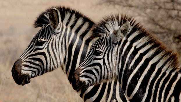https://sandipanweb.files.wordpress.com/2018/07/zebras.jpg?w=150 150w, https://sandipanweb.files.wordpress.com/2018/07/zebras.jpg?w=300 300w” sizes=”(max-width: 622px) 100vw, 622px” />

Output with edges detected with LOG + zero-crossing at different sigma scales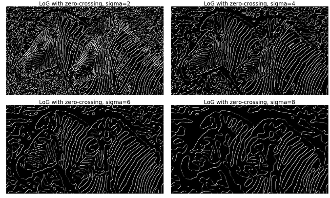
https://sandipanweb.files.wordpress.com/2018/07/zera_log_zc.png?w=1352 1352w, https://sandipanweb.files.wordpress.com/2018/07/zera_log_zc.png?w=150 150w, https://sandipanweb.files.wordpress.com/2018/07/zera_log_zc.png?w=300 300w, https://sandipanweb.files.wordpress.com/2018/07/zera_log_zc.png?w=768 768w, https://sandipanweb.files.wordpress.com/2018/07/zera_log_zc.png?w=1024 1024w” sizes=”(max-width: 676px) 100vw, 676px” />

With another input image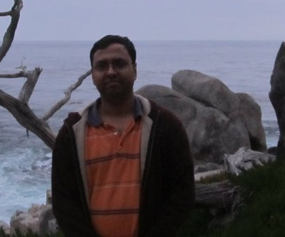
https://sandipanweb.files.wordpress.com/2018/07/me6.jpg?w=150 150w, https://sandipanweb.files.wordpress.com/2018/07/me6.jpg?w=300 300w” sizes=”(max-width: 399px) 100vw, 399px” />

Output with edges detected with LOG + zero-crossing at different sigma scales

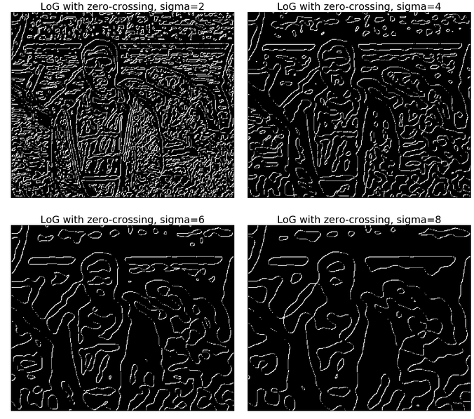https://sandipanweb.files.wordpress.com/2018/07/me6_log_zc.png?w=1352 1352w, https://sandipanweb.files.wordpress.com/2018/07/me6_log_zc.png?w=150 150w, https://sandipanweb.files.wordpress.com/2018/07/me6_log_zc.png?w=300 300w, https://sandipanweb.files.wordpress.com/2018/07/me6_log_zc.png?w=768 768w, https://sandipanweb.files.wordpress.com/2018/07/me6_log_zc.png?w=1024 1024w” sizes=”(max-width: 676px) 100vw, 676px” />

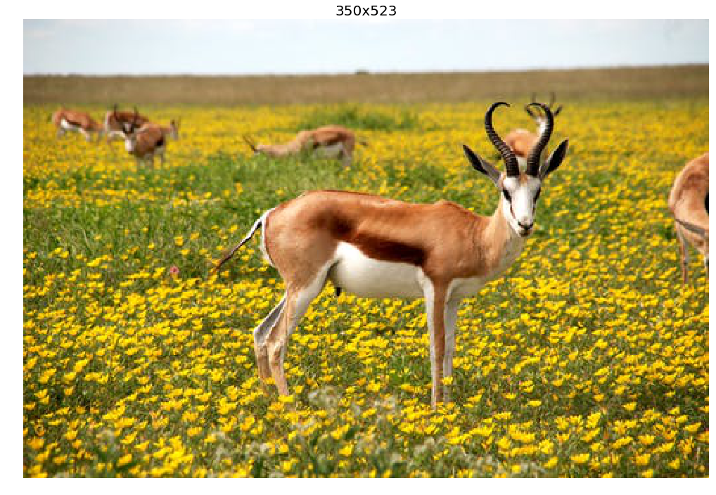
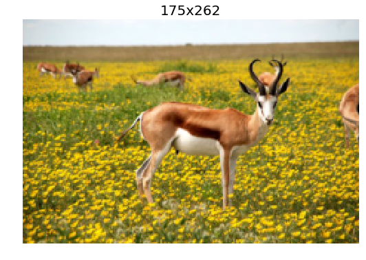
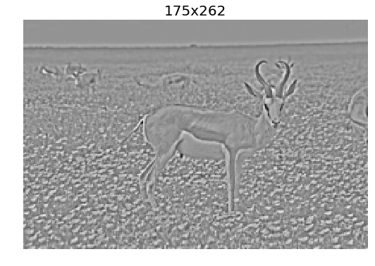
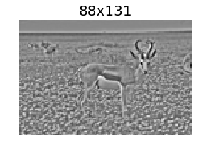
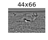
Constructing the Gaussian Pyramid with scikit-image transform module’s reduce function and Laplacian Pyramid from the Gaussian Pyramid and the expand function

The Gaussian Pyramid can be computed with the following steps:

Start with the original image.
Iteratively compute the image at each level of the pyramid first by smoothing the image (with gaussian filter) and then downsampling it .
Stop at a level where the image size becomes sufficiently small (e.g., 1×1).

The Laplacian Pyramid can be computed with the following steps:

Start with the Gaussian Pyramid and with the smallest image.
Iteratively compute the difference image in between the image at the current level and the image obtained by first upsampling and then smoothing the image (with gaussian filter) from the previous level of the Gaussian Pyramid.
Stop at a level where the image size becomes equal to the original image size.

The next python code shows how to create a Gaussian Pyramid from an image.

[code language=’python’] import numpy as np import matplotlib.pyplot as plt from skimage.io import imread from skimage.color import rgb2gray from skimage.transform import pyramid_reduce, pyramid_expand, resize def get_gaussian_pyramid(image): rows, cols, dim = image.shape gaussian_pyramid = [image] while rows&amp;amp;amp;amp;amp;amp;amp;gt; 1 and cols &amp;amp;amp;amp;amp;amp;amp;gt; 1: image = pyramid_reduce(image, downscale=2) gaussian_pyramid.append(image) print(image.shape) rows //= 2 cols //= 2 return gaussian_pyramid def get_laplacian_pyramid(gaussian_pyramid): laplacian_pyramid = [gaussian_pyramid[len(gaussian_pyramid)-1]] for i in range(len(gaussian_pyramid)-2, -1, -1): image = gaussian_pyramid[i] – resize(pyramid_expand(gaussian_pyramid[i+1]), gaussian_pyramid[i].shape) laplacian_pyramid.append(np.copy(image)) laplacian_pyramid = laplacian_pyramid[::-1] return laplacian_pyramid image = imread(‘../images/antelops.jpeg’) gaussian_pyramid = get_gaussian_pyramid(image) laplacian_pyramid = get_laplacian_pyramid(gaussian_pyramid) w, h = 20, 12 for i in range(3): plt.figure(figsize=(w,h)) p = gaussian_pyramid[i] plt.imshow(p) plt.title(str(p.shape[0]) + ‘x’ + str(p.shape[1]), size=20) plt.axis(‘off’) w, h = w / 2, h / 2 plt.show() w, h = 10, 6 for i in range(1,4): plt.figure(figsize=(w,h)) p = laplacian_pyramid[i] plt.imshow(rgb2gray(p), cmap=’gray’) plt.title(str(p.shape[0]) + ‘x’ + str(p.shape[1]), size=20) plt.axis(‘off’) w, h = w / 2, h / 2 plt.show() [/code]

Some images from the Gaussian Pyramid

Some images from the Laplacian Pyramid

Blending images with Gaussian and Laplacian pyramids

Here is the algorithm:

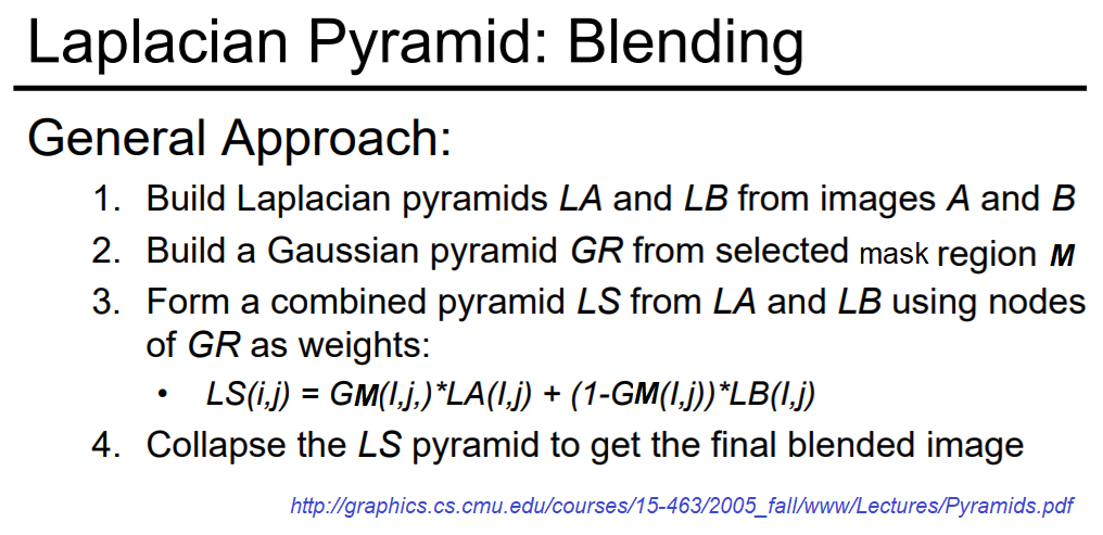
Blending the following input images A, B with mask image M

Input Image A (Goddess Durga)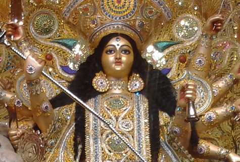 madurga1

Input Image B (Lord Shiva)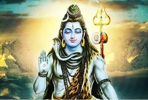
mahadeb

Mask Image M

with the following python code creates the output image I shown below

[code language=’python’] A = imread(‘../images/madurga1.jpg’)/255 B = imread(‘../images/mahadeb.jpg’)/255 M = imread(‘../images/mask1.jpg’)/255 # get the Gaussian and Laplacian pyramids, implement the functions pyramidA = get_laplacian_pyramid(get_gaussian_pyramid(A)) pyramidB = get_laplacian_pyramid(get_gaussian_pyramid(B)) pyramidM = get_gaussian_pyramid(M) pyramidC = [] for i in range(len(pyramidM)): im = pyramidM[i]*pyramidA[i] + (1-pyramidM[i])*pyramidB[i] pyramidC.append(im) # implement the following function to construct an image from its laplacian pyramids I = reconstruct_image_from_laplacian_pyramid(pyramidC) [/code]

Output Image I (Ardhanarishwar)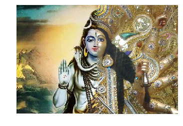
The following animation shows how the output image is formed: