MMS • RSS
Article originally posted on Data Science Central. Visit Data Science Central
Summary: Exceptions sometimes make the best rules. Here’s an example of well accepted variable reduction techniques resulting in an inferior model and a case for dramatically expanding the number of variables we start with.
 One of the things that keeps us data scientists on our toes is that the well-established rules-of-thumb don’t always work. Certainly one of the most well-worn of these rules is the parsimonious model; always seek to create the best model with the fewest variables. And woe to you who violate this rule. Your model will over fit, include false random correlations, or at very least will just be judged to be slow and clunky.
Certainly this is a rule I embrace when building models so I was surprised and then delighted to find a well conducted study by Lexis/Nexis that lays out a case where this clearly isn’t true.
A Little Background
In highly regulated industries like insurance and lending the variables that are allowed for use are highly regulated as are the modeling techniques. Techniques are generally limited to those that are highly explainable, mostly GLM and simple decision trees. Data can’t include anything that is overtly discriminatory under the law so, for example, race, sex, and age can’t be used, or at least not directly. All of this works against model accuracy.
Traditionally what agencies could use to build risk models has been defined as ‘traditional data’, that which the consumer has submitted with their application and the data that can be added from the major credit rating agencies. In this last case Experian and the others offer some 250 different variables and except for those that are specifically excluded by law, this seems like a pretty good sized inventory of predictive features.
But in the US and especially abroad the market contains many ‘thin-file’ or ‘no-file’ consumers who would like to borrow but for which traditional data sources simply don’t exist. Millennials feature in this group because their cohort is young and doesn’t yet have much borrowing or credit history. But also in this group are the folks judged to be marginal credit risks, some of whom could be good customers if only we knew how to judge the risk.
Enter the World of Alternative Data
‘Alternative data’ is considered to be any data not directly related to the consumer’s credit behavior, basically anything other than the application data and consumer credit bureau data. A variety of agencies are prepared to provide it and it can include:
- Transaction data (e.g. checking account data)
- Telecom/utility/rent data
- Social profile data
- Social network data
- Clickstream data
- Audio and text data
- Survey data
- Mobile app data
As it turns out lenders have been embracing alternative data for the last several years and see real improvements in their credit models, particularly at the low end of the scores. Even the CFPB has provisionally endorsed this to bring credit to the underserved.
 From a Data Science Perspective
From a data science perspective, in this example we started out with on the order of 250 candidate features from ‘traditional data’, and now, using ‘alternative data’ we can add an additional 1,050 features. What’s the first thing you do when you have 1,300 candidate variables? You go through the steps necessary to identify only the most predictive variables and discard the rest.
Here’s Where It Gets Interesting
Lexis/Nexis, the provider of the alternative data, set out to demonstrate that a credit model built on all 1,300 features was superior to one built on only 250 traditional features. The data was drawn from a full-file auto lending portfolio of just under 11 million instances. You and I might have concluded that even 250 was too many but in order to keep the test rigorous they introduced these constraints.
- The technique was limited to forward stepwise logistic regression. This provided clear univariate feedback on the importance of each variable.
- Only two models would be compared, one with the top 250 most predictive attributes and the other with all 1,300 attributes. This eliminated any bias from variable selection that might be introduced by the modeler.
- The variables for the 250 var model were selected by ranking the predictive power of each variables correlation to the dependent variable. As it happened all of the alternate variables fell outside the top 250 with the highest ranking 296th.
- The models were created with the same overall data prep procedures such as binning rules.
What Happened
As you might expect, the first and most important variable was the same for both models but began to diverge at the second variable. The second variable in the 1,300 model was actually 296th based on the earlier predictive power analysis.
When the model was completed the alternative data made up 25% of the model’s accuracy although none would have been included based on the top 250 predictive variables.
The KS (Kolmogorov-Smirnov) statistic was 4.3% better for the 1,300 model compared to the 250 model.
The Business Importance
The distribution of scores and charge offs for each models was very similar but in the bottom 5% of scores things changed. There was a 6.4% increase in the number of predicted charge offs in this bottom group.
Since the distributions are the essentially the same this can be seen as higher scores that might have been rated credit worthy migrating into the lowest categories of credit worthiness allowing better decisions about denial or pricing based on risk. Conversely it appears that some lowest rated borrowers were given a boost with the additional data.
That also translates to a competitive advantage for those using the alternative data compared to those who don’t. You can see the original study here.
There are Four Lesson for Data Scientists Here
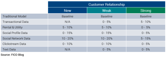
- Think outside the box and consider the value of a large number of variables when first developing or refining your model. It wasn’t until just a few years ago that the insurance industry started looking at alternative data and on the margin it has increased accuracy in important ways. FICO published this chart showing the relative value of each category of alternative data strongly supporting using more variables.
- Be careful about using ‘tried and true’ variable selection techniques. In the Lexis/Nexis case starting the modeling process with variable selection based on univariate correlation with the dependent variable was misleading. There are a variety of other techniques they could have tried.
- Depending on the amount of prep, it still may not be worthwhile expanding your variables so dramatically. More data always means more prep means more time which in a commercial environment you may not have. Still, be open to exploration.
- Adding ‘alternate source’ data to your decision making can be a two edged sword. In India, measures as obscure as how often a user charges his cell phone or its average charge level has proven to be predictive. In that credit-starved environment these innovative measures are welcomed when they provide greater access to credit.
On the other hand just this week a major newspaper in England published as expose of comparative auto insurance rates where it discovered that individuals applying with a Hotmail account were paying as much as 7% more than those with Gmail accounts. Apparently British insurers had found a legitimate correlation between risk and this alternative data. It did not sit well with the public and the companies are now on the defensive.
About the author: Bill Vorhies is Editorial Director for Data Science Central and has practiced as a data scientist since 2001. He can be reached at:
