Month: March 2025

Posted on mongodb google news. Visit mongodb google news

Temporal Technologies, a Seattle, WA-based inventor of open-source durable execution platforms Temporal.io and Temporal Cloud, raised $146M in funding, at $1.72 Billion valuation.

The round was led by Tiger Global with participation from StepStone Group, Amplify Partners, Index Ventures, MongoDB Ventures, Sequoia Capital, Conversion Capital, Hanwha Next Generation Opportunity Fund, and 137 Ventures.

The company intends to use the funds to accelerate product development for its enterprise-grade managed service Temporal Cloud and expand the reach of its durable execution platform beyond mission-critical workloads in payments, e-commerce, air travel, and disruptive digitally native companies, and into AI use cases of all types.

Temporal provides an open-source durable execution platform that guarantees the execution of complex workflows even in the face of system failures and allows developers to focus entirely on business logic. Its polyglot capabilities allow orchestration across multiple programming languages, making it ideal for both traditional enterprise applications and next-generation AI workloads. Temporal Cloud, the company’s managed service backed by the originators of the project, has been adopted by over 2,500 customers globally,

Temporal recently added B2B software veteran Jim Cyb as President to lead go-to-market efforts and announced the appointment of Sahir Azam, Chief Product Officer of MongoDB, as its first independent board member.

FinSMEs

31/03/2025

Article originally posted on mongodb google news. Visit mongodb google news

Article originally posted on InfoQ. Visit InfoQ

Transcript

Stern: We’re going to talk about topologies for cost-saving autoscaling. Just to get you prepared, it’s not going to be like I’m showing you, this is how you’re going to autoscale your environment, but rather ways to think about autoscaling, and what are the pitfalls and the architecture of OpenSearch that limit autoscaling in reality. I’m going to start talking about storing objects, actual objects, ice-core samples. Ice-core samples are these cylinders drilled from ice sheets or glaciers, and they provide us a record of Earth’s climate and environment.

The interesting thing, I believe, and relevant to us in these ice-core samples is that when they arrive at the storage facility, they are parsed. If you think about it, this is probably the most columnar data of any columnar data that we have. It’s a literal column. It’s sorted by timestamp. You have the new ice at the top and the old ice at the bottom. The way the scientific community has decided to parse this data is in the middle of the slide. It’s very clear to them that this is how they want it parsed. This person managing the storage facility is going to parse the data that way, all of it. Because the scientific community has a very narrow span of inquiry regarding this type of data, it is easy to store it. It is easy to make it very compact. You can see the storage facility is boring. It’s shelves. Everything is condensed. A visitor arriving at the facility has an easy time looking for things. It’s very well-sorted and structured.

If we take a hypothetical example of lots of visitors coming, and the person here who is managing the storage facility wants to scale out, he wants to be able to accommodate many more visitors at a time. What he’ll do is he’ll take all those ice-core samples, and cut them in half. That’s just time divided by two. That’s easy. Add a room. Put all these halves in another room. You can spread out the load. The read load will be spread out. It really makes things easy. It’s practically easy to think about how you’d scale out such a facility. Let’s talk about a different object storage facility, like a museum, where we don’t really know what kind of samples are coming in. If you have a new sample coming in, it could be a statue, it could be an archaeological artifact, it could be a postmodern sculpture of the Kraken or dinosaur bones. How do we index these things in a way that they’re easy to search? It’s very hard.

One of the things that’s interesting is that a visitor at a museum has such a wide span of inquiry. Like, what are they going to ask you? Or a person managing the museum, how does he index things so that they’re easily queryable? What if someone wants the top-k objects in the museum? He’ll need these too, but they’re from completely different fields. When your objects are unstructured, it’s very hard to store them in a way that is scalable. If we wanted to scale our museum for this hypothetical situation where many visitors are coming, it’s hard to do. Would we have to take half of this dinosaur skeleton and put it in another room? Would we take samples from each exhibit and make a smaller museum on the side? How do you do this? In some real-world cases, there’s a lot of visitors who want to see a specific art piece and it’s hard. How do you scale the Mona Lisa? You cannot. It’s just there and everybody is going to wait in line and complain about it later.

Similarly, to OpenSearch, you can scale it. That’s adding nodes. It’s a mechanical thing. You’re just going to add some machines. Spreading the load when your data is unstructured is difficult. It’s not a straightforward answer. This is why in this particular type of system and in Elasticsearch as well, you don’t have autoscaling native to the software.

Background

I’m Amitai Stern. I’m a member of the Technical Steering Committee of the OpenSearch Software Foundation, leading the OpenSearch software. I’m a tech lead at Logz.io. I manage the telemetry storage team, where we manage petabytes of logs and traces and many terabytes of monitoring and metric data for customers. Our metrics are on Thanos clusters, and everything else that I mentioned, logs and traces, are all going to be stored on OpenSearch clusters.

What Is OpenSearch?

What is OpenSearch? OpenSearch is a fork of Elasticsearch. It’s very similar. It’s been a fork for the last three years. The divergence is not too great. If you’re familiar with Elasticsearch, this is very much relevant as well. OpenSearch is used to bring order to unstructured data at scale. It’s the last line over here. It is a fork of Elasticsearch. Elasticsearch used to be open source. It provided an open-source version, and then later they stopped doing that. OpenSearch is a fork that was primarily driven by AWS, and today it’s completely donated to the Linux Foundation. It’s totally out of their hands at this point.

OpenSearch Cluster Architecture

OpenSearch clusters are monolithic applications. You could have it on one node. From here on in the talk, this rounded rectangle will represent a node. A node in OpenSearch can have many roles. You can have just one and it’ll act as its own little cluster, but you could also have many and they’ll interact together. That’s what monolithic applications are. Usually in the wild, we’ll see clusters divided into three different groups of these roles. The first one would be a cluster manager. The cluster manager nodes are managing the state where indexes are, creating and deleting indexes. There’s coordinating nodes, and they’re in charge of the HTTP requests. They’re like the load balancer for the cluster. Then there’s the data nodes. This is the part that we’re going to want to scale. Normally this is where the data is. The data is stored within a construct called an index. This index contains both the data and the inverted index that makes search fast and efficient.

These indices are split up, divided between the data nodes in a construct called a shard. Shards go from 0 to N. A shard is in fact a Lucene index, just to make things a little bit confusing. You already used the term index, so you don’t need to remember that. They’re like little Lucene databases. On the data nodes are three types of pressure if you’re managing one. You’re managing your cluster. You have the read pressure, all the requests coming in to pull data out as efficiently as possible and quickly as possible, and this write pressure of all these documents coming in. There’s the third pressure when you’re managing a cluster, which is the financial one. Since if your read and writes are fairly low, you’ll get a question from your management or from the CFO like, what’s going on? These things cost a lot of money: all this disk space, all the memory, and CPU cores. It’s three types of pressure.

Why Autoscale?

Let’s move on to why would you even autoscale? Financially, cluster costs a lot of money. We want to reduce the amount of nodes that we have. What if we just had enough to handle the scale? This blue line will be the load. The red line is the load that we can accommodate for with the current configuration. Leave it vague that way. Over-provisioned is blue, and under-provisioned is the red over there. If we said the max load is going to be x, and we’re just going to say, we just provision for there. We’ll have that many nodes. The problem would be that we’re wasting money. This is good in some cases if you have the money to spend. Normally, we’re going to try and reduce that. You opt for manual scaling. Manual scaling is the worst of both worlds. You wait too long to scale up because something’s happening to the system. It’s bad performance. You scale up.

Then you’re afraid to scale down at this point because a second ago, people were complaining, so you’re going to wait too long to scale down. It’s really the worst. Autoscaling is following that curve automatically. That’s what we want. This is the holy grail, some line that follows the load. When we’re scaling OpenSearch, we’re scaling hardware. We have to think about these three elements that we’re scaling. We’re going to scale disk. We’re going to scale memory. We’re going to scale CPU core. These are the three things we want to scale. The load splits off into these three. Read load doesn’t really affect the disk. You can have a lot of read load or less read load. It doesn’t mean you’re going to add disk. We’re going to focus more on the write load and its effects on the cluster, because it affects all three of these components. If there’s a lot of writes, we might need to add more disk, or we might need more CPU cores because the type of writing is a little more complex, or we need more memory.

Vertical and Horizontal Scaling

I have exactly one slide devoted to vertical scaling because when I was going over the talk with other folks, they said, what about vertical scaling? Amazon, behind the scenes when they’re running your serverless platform, they’re going to vertically scale it first. If you have your own data center, it could be easy to do that relatively. Amazon do this because they have the capability to vertically scale easily. If you’re using a cloud, it’s harder. When you scale up, usually you go from one set of machines to the next scale of machines. It means you have to stop that machine and move data. That’s not something that’s easily done normally. Vertically scaling, for most intent and purposes in most companies, is really just the disk. That is easy. You can increase the number of EBS instances. You can increase the disk over there. Horizontal scaling is the thing you need to know how to do.

If you’re managing and maintaining clusters, you have to know how to do this. OpenSearch, you just have to add a node, and it gets discovered by the cluster, and it’s there. Practically, it’s easy. There’s a need to do this because of the load, the changing load. There’s an expectation, however, that when you add a node, the load will just distribute. This is the case in a lot of different projects. Here, similar to the example with the museum, it’s not the case. You have to learn how the load is spread out. You have to actually change that as well. How you’re maintaining the data, you have to change that as you are adding nodes.

If the load is disproportionately hitting one of the nodes, we call that a hotspot. Any of you familiar with what hotspots are? You get a lot of load on one of those nodes, and then writes start to lag. Hotspots are a thing we want to avoid. Which moves us into another place of, how do we actually distribute this data so it’s going to all these nodes in the same fashion and we’re not getting these hotspots? When we index data into OpenSearch, each document gets its own ID. That ID is going to be hashed, and then we’re going to do a Mod of N. N being the number of shards. In this example, the Mod is something that ends with 45, and Mod 4, because we have 4 shards. That would be equal to 1, so it’s going to go to shard number 1. If you have thousands of documents coming in, each with their own unique ID, then they’re going to go to these different shards, and it more or less balances out. It works in reality.

If we wanted to have the capability to just add a shard, make the index just slightly bigger, why can’t we do that? The reason is this hash Mod N. If we were to potentially add another shard, our document is now stored in shard number 1, and we want it to scale up, so we extended the index just a bit.

The next time we want to search for that ID, we’re going to do hash Mod to see where it is. N just changed, it’s 5 and not 4. We’re looking for the document in a different shard, and it is now gone. That’s why we have a fixed number of shards in our indices. We actually can’t change that. When you’re scaling OpenSearch, you have to know this. You can’t just add shards to the index. You have to do something we call a rollover. You take the index that you’re writing to, and you add a new index with the same aliases. You’re going to start writing to the new index atomically. This new index would have more shards. That’s the only way to really increase throughput.

Another thing that’s frustrating when you’re trying to horizontally scale a cluster is that there’s shared resources. Each of our data nodes is getting hit with all these requests to pull data out and at the same time to put data in. If you have a really heavy query with a leading wildcard, RegEx, something like that, hitting one or two of your nodes, the write throughput is going to be impacted. You’re going to start lagging in your writes. Why is this important to note? Because autoscaling, often we look at the CPU and we say, CPU high at nodes. That could be because of one of these two pressures. It could be the write pressure or the read. If it’s the read, it could be momentary, and you just wasted money by adding a lot of nodes.

On the one hand, we shouldn’t look at the CPU, and we might want to look at the write load and the read load. On the other hand, write load and read load could be fine, but you have so many shards packed in each one of your nodes because you’ve been doing all these rollover tasks that you get out of memory. I’m just trying to give you the feeling of why it’s actually very hard to do this thing where you’re saying, this metric says scale up.

Horizontally Scaling OpenSearch

The good news is, it’s sometimes really simple. It does come at a cost, similarly to eating cake. It is still simple. If the load is imbalanced on one of those three different types, disk, memory, or CPU, we could add extra nodes, and it will balance out, especially if it’s disk. Similarly, if the load is low on all three, it can’t be just one, on all three of those, so low memory, low CPU, low disk, we can remove nodes. That’s when it is simple, when you can clearly see the picture is over-provisioned or under-provisioned. I want to devote the rest of the talk to when it’s actually complicated because the easy is really easy. Let’s assume that we’re looking at one of those spikes, the load goes up and down. Let’s say we want to say that when we see a lot of writes coming in, we want to roll over. When they go down, we want to roll over again because we don’t want to waste money. The red is going to say that the writes are too high. We’re going to roll over.

Then we add this extra node, and so everything is ok. Then the writes start to go down, we’re wasting money at this point. There’s 20% load on each of these nodes. If we remove a node, we get a hotspot because now we just created a situation where 40% is hitting one node, a disproportionate amount of pressure on one. That’s bad. What do we do? Do another rollover task, and now it’s 25% to each node. We could do this again and again on each of these. If it’s like a day-night load, you’d have way too many shards already in your cluster, and you’d start hitting out of memory. Getting rid of those extra shards is practically hard. You have to find a way to either do it slowly by changing to size-based retention, or you can do merging of indexes, which you can do, but it’s very slow. It takes a lot of CPU.

Cluster Topologies for Scaling

There is a rather simple way to overcome this problem, and that is to overshard. Rather than have shards spread out one per node, I could have three shards per node. Then, when I want to scale, I’ll add nodes and let those shards spread out. The shards are going to take up as much compute power as it can from those new nodes, so like hulking out. That’s the concept. However, finding the sweet spot between oversharding and undersharding becomes hard. It’s difficult to calculate. In many cases, you’d want to roll over again into an even bigger index. I’m going to suggest a few topologies for scaling in a way that allows us to really maintain this sweet spot between way too many, way too few shards. The first kind is what I’d call a burst index.

As I mentioned earlier, each index has a write alias. That’s where you’re going to atomically be writing. You can change this alias, and it’ll switch over to whatever index you point to. It’s an important concept to be familiar with if you’re managing a cluster. What we’re suggesting is to have these burst indices prepared in case you want to scale out. They can be maintained for weeks, and they will be that place where you direct traffic when you need to have a lot of it directed there. That’s what we would do. We just change the write alias to the write data stream. That would look something like this. There’s an arbitrary tag, a label we can give nodes called box_type. You could tell an index to allocate its shards on a specific box_type or a few different box_types. The concept is you have burst type, the box_type: burst, and you have box_type: low.

As long as you have low throughput in your writes, and again, that is probably the best indicator of I need more nodes, is the write throughput. If we have a low throughput on the writes, we don’t need our extra nodes. The low write throughput index is allocated to indexes that have the low box_type. If throughout the day the throughput is not so low and we anticipate that we’re going to have a spike, and this, again, it’s so tailored to your use case that I can’t tell you exactly what that is. If you see, in many cases, it is that the write throughput is growing on a trend, then what you do is you add these extra nodes. You don’t need to add nodes that are as expensive as the other ones. Why? Because you don’t intend to have that amount of disk space used on them. They’re temporary. You could have a real small and efficient disk there on these new box_types. You create the new ones. The allocation of our burst index says it can be on either low or burst or both. All you have to do is tell that index that you’re allowed to have total shards per node, 1.

Then it automatically will spread out to all of these nodes. At this point, you’re prepared for the higher throughput, and you switch the write alias to be the high throughput index. This is the burst index type. As it goes down, you can move the shards back by doing something called exclude of the nodes. You just exclude these nodes, and shards just fly off of it to other nodes. Then you remove them. This is the first form of autoscaling. It works when you don’t have many tenants on your cluster. If you have one big index, and it may grow or shrink, this makes sense.

However, in some cases, we have many tenants, and they’re doing many different things all at the same time. Some throughputs spike, when others will go down. You don’t want to be in a situation where you’re having your cluster tailored just for the highest throughput tenant. Because then, again, you are wasting resources.

Which brings me to the second and last topology that I want to discuss here, which is called the burst cluster. It is very similar to the previous one, but the difference is big. We’re not just changing the index that we’re going to within the cluster, we’re changing the direction to a completely different cluster. We wouldn’t be using the write alias, we would be diverting traffic. It would look something like this. If each of these circles is a cluster, and each of them have that many nodes, why would we have a 10, and a 5, and a 60? The reason is we’d want to avoid hotspots. You should fine-tune your clusters initially for your average load. The average load for a low throughput might be 5 nodes, so you want only 5 shards. For a higher throughput, you want a 10-node cluster, so you have 10 shards each. If you’re suffering from hotspots, all you have to do to fix that is spread the shards perfectly on the cluster. That means zero hotspots.

In this situation, we’ve tailored our system so that on these green clusters, the smaller circles, they’re fine-tuned for the exact amount of writes that we’re getting. Then one of our tenants spikes while the others don’t. We move only that tenant to send all their data, we divert it to the 60-node cluster, capable of handling very high throughputs, but not capable of handling a lot of disk space. It’s not as expensive as six times these 10-node clusters. It is still more expensive. Data is being diverted to a totally different environment. We use something called cross-cluster search in order to search on both. From the perspective of the person running the search, nothing has changed at any point. It’s completely transparent for them.

In terms of the throughput, nothing has changed. They’re sending much more data, but they don’t get any lag, whoever is sending it. All the other tenants don’t feel it. There are many more tenants on this 10-node cluster, and they’re just living their best life over there. You could also have a few tenants sending to this 60-node cluster. You just have to manage how much disk you’re expecting to fill at that time of the burst. A way to make this a little more economical is to have one of your highest throughput tenants always on the 60-node cluster. You still maintain a reason to have them up when there’s no high throughput tenants on these other clusters. This is a way to think of autoscaling in a way that is a bit outside of the box and not just adding nodes to a single cluster. It is very useful, if you are running a feature that is not very used in OpenSearch, but is up and coming, called searchable snapshots.

If you’re running searchable snapshots, all your data is going to be on S3, and you’re only going to have metadata on your cluster. The more nodes you have that are searching S3, the better. They can be small nodes with very small disk, and they could be searching many terabytes on S3. If you have one node with a lot of disk trying to do that, the throughput is going to be too low and your search is going to be too slow. If you want to utilize these kinds of features where your data is remote, you have to have many nodes. That’s another reason to have such a cluster just up and running all the time. You could use it to search audit data that spans back many years. Of course, we don’t want to keep it there forever.

A way to do that is just snapshot it to S3. Snapshots in OpenSearch are a really powerful tool. They’re not the same as they are in other databases. It takes the index as it is. It doesn’t do any additional compression, but it stores it in a very special way, so it’s easy to extract it and restore a cluster in case of a disaster. We would move the data to S3 and then restore it back into these original clusters that we had previously been running our tenants on. Then we could do a merge task. Down the line, when the load is low, we could merge that data into smaller indexes if we like. Another thing that happens usually in these kinds of situations is that you have retention. Once the retention is gone, just delete the data, which is great. Especially if you’re in Europe, you have to delete it right on time. This is the burst cluster topology.

Summary

There are three different resources that we want to be scaling. You have to be mindful when you’re maintaining your cluster which one is the one that causes the pressure. If you have very long retention, then disk space. You have to start considering things like searchable snapshots or maintaining maybe a cross-cluster search where you have just data sitting on a separate cluster that’s just accumulating in very large disks, whereas your write load is on a smaller cluster. That’s one possibility. If it’s memory or CPU, then you would definitely have to add stronger machines. We have to think about these things ahead of time. Some of them are a one-way door.

If you’re using AWS and you add to your disk space, in some cases, you may find it difficult to reduce the disk space again. This is a common problem. When I say that, the main reason it is is because when you want to reduce a node, you have to shift the data to the other nodes. In certain cases, especially after you’ve added a lot of disk, that can take a lot of time. Some of them are a one-way door. Many of them require a restart of a node, which is potential downtime. We talked about these two topologies, I’ll remind you, the burst index and the burst cluster, which are very important to think about as completely different options. I like to highlight that that first option that I gave, the hulking out, like the oversharding proposition, is also viable for many use cases.

If you have a really easy trend that you can follow, your data is just going up and down, and it’s the same at noon. People are sending 2x. Midnight, it goes down to half of that. It keeps going up and down. By all means, have a cluster that has 10 nodes with 20 shards on it. When you hit that afternoon peak, just scale out and let it spread out. Then when it gets to the evening, then scale down again. If that’s your use case, you shouldn’t be implementing things that are this complex. You should definitely use the concept of oversharding, which is well-known.

Upcoming Key Features

I’d like to talk about some upcoming key features, which is different than when I started writing this presentation. These things changed. The OpenSearch Software Foundation, which supports OpenSearch, one of the things that’s really neat is that from it being very AWS-centric, it has become much more widespread. There’s a lot of people from Uber and Slack, Intel, Airbnb, developers starting to take an interest and developing things within the ecosystem. They’re changing it in ways that will benefit their business.

If that business is as big as Uber, then the changes are profound. One of the changes that really affects autoscaling is read/write separation. That’s going to come in the next few versions. I think it’s nearly beta, but a lot of the code is already there. I think this was in August when I took this screenshot, and it was a 5 out of 11 tasks. They’re pretty much there by now. This will allow you to have nodes that are tailored for write and nodes that are tailored for read. Then you’re scaling the write, and you’re scaling the read separately, which makes life so much more simple.

The other one, which is really cool, is streaming ingestion. One of the things that really makes it difficult to ingest a lot of data all at once is that today, in both Elasticsearch and OpenSearch, we’re pushing it in. The index is trying to do that, trying to push the data and ingest it. The node might be overloaded, in which case the shard will just say, I’m sorry, CPU up to here, and you get what is called a write queue. Once that write queue starts to build, someone’s going to be woken up, normally. If you’re running observability data, that’s a wake-up call. In pull-based, what you get is the shard is hardcoded to listen and retrieve documents from a particular partition in for example, Kafka. It would be pluggable, so it’s not only Kafka.

Since it’s very common, let’s use Kafka as an example. Each shard will read from a particular partition. A topic would represent a tenant. You could have a shard reading from different partitions from different topics, but per topic, it would be one, so shard 0 from partition 0. What this gives us is the capability for the shard to read as fast as it can, which means that you don’t get the situation of a write queue, because it’s reading just as fast as it possibly can, based on the machine, wherever you put it. If you want to scale, in this case, it’s easy. You look at the lag in Kafka. You don’t look at these metrics in terms of the cluster. The metrics here are much easier. Is there a lag in Kafka? Yes. I need to scale. Much easier. Let’s look at CPU. Let’s look at memory. Let’s see if the shards are balanced. It’s much harder to do. In this case, it will make life much easier.

Questions and Answers

Participant 1: I had a question about streaming ingestion. Beyond just looking at a metric, at the lag in Kafka, does that expose a way to know precisely up to which point in the stream this got in the document? We use OpenSearch in a bunch of places where we need to know exactly what’s available in the index so that we can propagate things to other systems.

Stern: It is an RFC, a request for comments.

Participant 1: There’s not a feature yet.

Stern: Right now, it’s in the phase of what we call a feature branch, where it’s being implemented in a way that it’s totally breakable. We’re not going to put that in production. If you have any comments like that, please do comment in the GitHub. That would be welcome. It’s in the exact phase where we need those comments.

Participant 2: This is time-series data. Do you also roll your indexes by time, like quarterly or monthly, or how do you combine this approach with burst indexes with a situation where you have indexes along the time axis.

Stern: If it’s retention-based? One of the things you can do is you have the burst index. You don’t want it to be there for too long. The burst index, you want it to live longer than the retention?

Participant 2: It’s not just the burst indexes, your normal indexes are separated by time.

Stern: In some cases, if your indexes are time-based and you’re rolling over every day, then you’re going to have a problem of too many shards if you don’t fill them up enough. You’ll have, basically, shards that have 2 megabytes inside them. It just inflates too much. If you have 365 days or two years of data, that becomes too many shards. I do recommend moving to size-based, like a hybrid solution of size-based, as long as it’s less than x amount of days, so that you’re not exactly on the date but better. Having said that, the idea is that you have your write alias pointed at the head. Then after a certain amount of time, you do a rollover task. The burst index, you don’t roll over, necessarily. That one, what you do instead of rolling over, you merge, or you do a re-index of that data into the other one. You can do that. It just takes a lot of time to do. You can do that in the background. There’s nitty-gritty here, but we didn’t go into that.

Participant 3: I think you mentioned separation of reading and writing. It’s already supported in OpenSearch Serverless in AWS. Am I missing something? The one that you are talking about, is it going to come for the regular OpenSearch, and it’s not yet implemented?

Stern: I don’t work at AWS. I’m representing open source. Both of these are going to be completely in open source.

Participant 3: That’s what I’m saying. It seems like it’s already there in version, maybe 2.13, 2.14, something like that. You mentioned it is a version that is coming, but I have practically observed that it’s already there, in Amazon serverless.

Stern: Amazon serverless is a fork of OpenSearch. It took a nice amount of engineers more than a year to separate these two things, these concepts of OpenSearch is a multi-application and having to read/write. A lot of these improvements, they’re working upstream. They like to add these special capabilities, like read/write separation. Then they contribute a lot of the stuff back into the open source. In some cases, you’ll have features already available in the Amazon OpenSearch offering, then later, it’ll get introduced into the OpenSearch open source.

Participant 3: The strategies that you explained just now, and they are coming, especially the second one, one with the Kafka thing, is there a plan?

Stern: Again, this is very early stage, the pull-based indexing. That one is at a stage where we presented the API that we imagine would be useful for this. We developed the concept of it’ll be pluggable, like which streaming service you’d use. It’s at a request for comments stage. I presented it because I am happy to present these things and ask for comments. If you have anything that’s relevant, just go on GitHub and say, we’re using it for this, and one-to-one doesn’t make sense to us. If that’s the case, then yes.

Participant 3: It can take about six months to a year?

Stern: That particular one, we’re trying to get in under a year. I don’t think it’s possible in six months. That’s a stretch.

Participant 4: I think this question pertains to both the burst index and the burst cluster solution. I think I understand how this helps for writing new documents. If you have an update or a delete operation, where you’re searching across your old index, or your normal index, and then either the burst index or the burst cluster, and that update or that delete is reflected in the burst cluster, how does that get rectified between those two?

Stern: One of the things you have to do if you’re maintaining these types of indexes, like a burst index, is you would want to have a prefix that signifies that tenant, so that any action you do, like a deletion, you’d say, delete based on these aliases. You have the capability of specifying either the prefix with a star in the end, like a wildcard. You could also give indexes, and it’s very common to do this, especially if it’s time-series data, to give a read alias per day. You have an index, and it contains different dates with the tenant ID connected to them. When you perform a search, that tenant ID plus November 18th, then that index is then made available for search. You can do the same thing when you’re doing operations like get for a delete. You can say, these aliases, I want to delete them, or I want to delete documents from them. It can go either to the burst cluster, or it could go to the indexes that have completely different names, as long as the alias points to the correct one.

The cluster means you have to really manage it. You have to have some place where you’re saying, this tenant has data here and there, and the date that I changed the tenant to be over there, and the date that I changed them back. It’s very important to keep track of those things. I wouldn’t do it within OpenSearch. A common mistake when you’re managing OpenSearch, is to say, I have OpenSearch, so I’m going to just store lots of information in it, not just the data that I built the cluster for. It should be a cluster for a thing and not for other things. Audit data should be separated from your observability data. You don’t want to put them in the same place.

Participant 5: A question regarding the burst clusters, as well as the burst nodes that you have. With clusters, how do you redirect the read load directly? Is the assumption that we do cross-cluster search? With OpenSearch dashboards in particular, when you have all your alerts and all that, and with observability data, you’re acquiring a particular set of indexes, so when you move the data around clusters, how do you manage the search?

Stern: For alerting, it is very difficult to do this if you’re managing alerting using just the index. If you use a prefix, it could work. If you’re doing cross-cluster search, the way that that feature works is that, in the cluster settings, you provide the clusters that it can also search on. Then when you run a search, if you’re doing it through Amazon service, it should be seamless. If you’re running it on your own, you do have to specify, instead of just search this index, it doesn’t know that it has to go to the other cluster. You have to say, within this cluster, and that cluster, and the other cluster, search for this index. You have to add these extra indexes to your search.

Participant 5: There is a colon mechanism where you put in. Basically, what you’re expecting here is, in addition to write, with read, we have to keep that in mind before spinning up a burst cluster.

Stern: You have to keep track where your data is when you’re moving it.

Participant 5: The second part of the question with burst nodes is, I’m assuming you’re amortizing the cost of rebalancing. Because whenever the node goes up and down, so your cluster capacity, or the CPU, because shards are moving around, and that requires CPU, network storage, these transport actions are happening. You’re assuming, as part of your capacity planning, you have to amortize that cost as well.

Stern: Yes. Moving a shard while it’s being written to, and it has already 100 gigs on it, moving that shard is a task that is just going to take time. You need high throughput now. It’s amortized, but it’s very common to do a rollover task with more shards when your throughput is big. It’s the same. You’d anyway be doing this. You’d anyway be rolling over to an index that has more shards and more capability of writing on more nodes. It’s sort of amortized.

Participant 5: With the rollover, you’re not moving the data, though. It’s new shards getting created.

Stern: Yes. We don’t want to move data when we’re doing the spread-out. That really slows things down.

See more presentations with transcripts

Article originally posted on InfoQ. Visit InfoQ

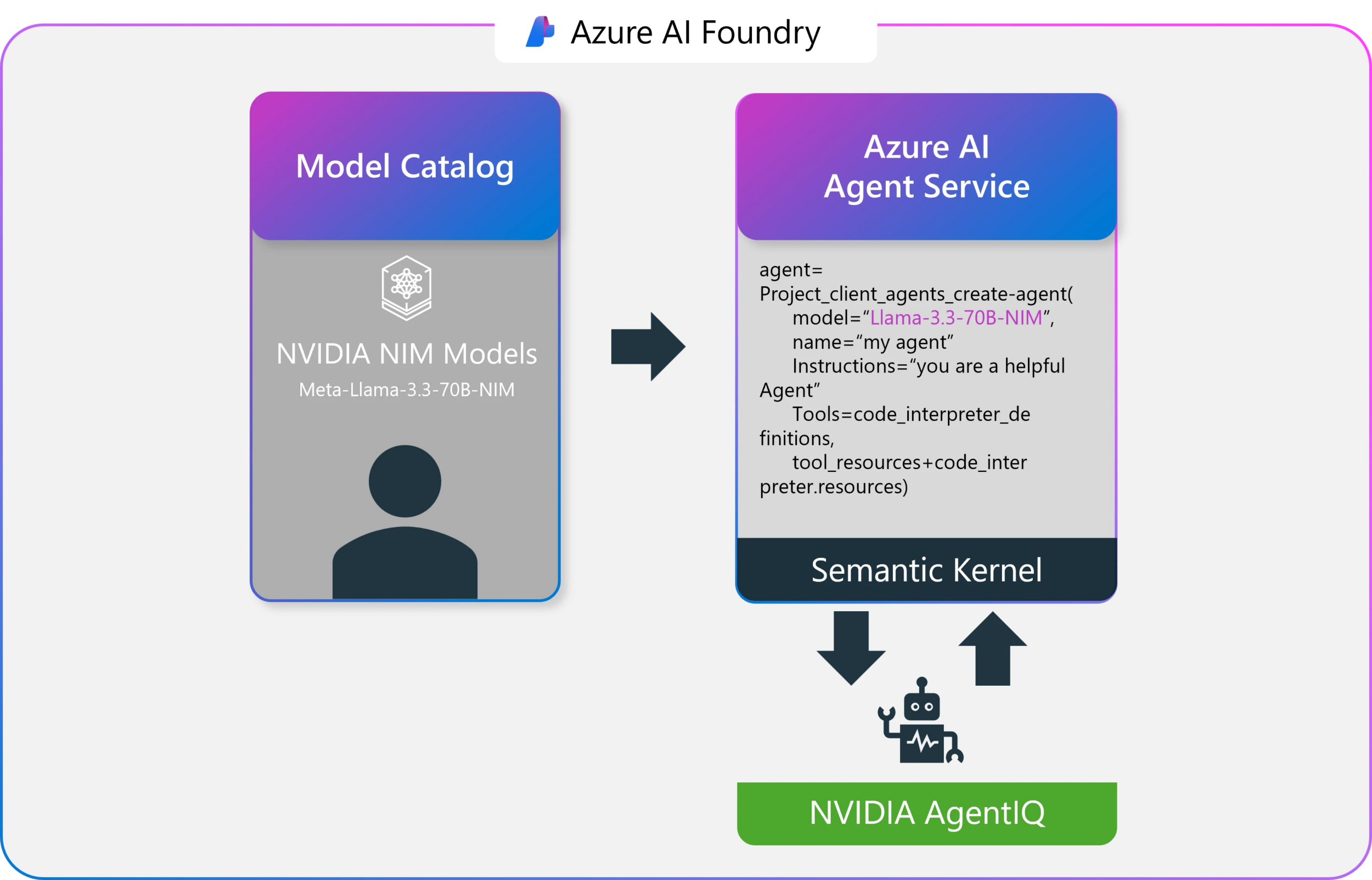
In collaboration with NVIDIA, Microsoft has announced the integration of NVIDIA NIM microservices and the NVIDIA AgentIQ toolkit into Azure AI Foundry. This strategic move aims to significantly accelerate the development, deployment, and optimization of enterprise-grade AI agent applications, promising streamlined workflows, enhanced performance, and reduced infrastructure costs for developers.

The integration directly addresses the often lengthy enterprise AI project lifecycles, extending from nine to twelve months. By providing a more efficient and integrated development pipeline within Azure AI Foundry, leveraging NVIDIA’s accelerated computing and AI software, the goal is to enable faster time-to-market without compromising the sophistication or performance of AI solutions.

NVIDIA NIM (NVIDIA Inference Microservices), a key component of the NVIDIA AI Enterprise software suite, offers a collection of containerized microservices engineered for high-performance AI inferencing. Built upon robust technologies such as NVIDIA Triton Inference Server, TensorRT, TensorRT-LLM, and PyTorch, NIM microservices provide developers with zero-configuration deployment, seamless integration with the Azure ecosystem (including Azure AI Agent Service and Semantic Kernel), enterprise-grade reliability backed by NVIDIA AI Enterprise support, and the ability to tap into Azure’s NVIDIA-accelerated infrastructure for demanding workloads. Developers can readily deploy optimized models, including Llama-3-70B-NIM, directly from the Azure AI Foundry model catalog with just a few clicks, simplifying the initial setup and deployment phase.

Once NVIDIA NIM microservices are deployed, NVIDIA AgentIQ, an open-source toolkit, takes center stage in optimizing AI agent performance. AgentIQ is designed to seamlessly connect, profile, and fine-tune teams of AI agents, enabling systems to operate at peak efficiency.

Daron Yondem tweeted on X:

NVIDIA’s AgentIQ treats agents, tools, and workflows as simple function calls, aiming for true composability: build once, reuse everywhere.

The toolkit leverages real-time telemetry to analyze AI agent placement, dynamically adjusting resources to reduce latency and compute overhead. Furthermore, AgentIQ continuously collects and analyzes metadata—such as predicted output tokens per call, estimated time to following inference, and expected token lengths—to dynamically enhance agent performance and responsiveness. The direct integration with Azure AI Foundry Agent Service and Semantic Kernel further empowers developers to build agents with enhanced semantic reasoning and task execution capabilities, leading to more accurate and efficient agentic workflows.

(Source: Dev Blog post)

Drew McCombs, vice president of cloud and analytics at Epic, highlighted the practical benefits of this integration in an AI and Machine Learning blog post, stating:

The launch of NVIDIA NIM microservices in Azure AI Foundry offers Epic a secure and efficient way to deploy open-source generative AI models that improve patient care.

In addition, Guy Fighel, a VP and GM at New Relic, posted on LinkedIn:

NVIDIA #AgentIQ will likely become a leading strategy for enterprises adopting agentic development. Its ease of use, open-source nature, and optimization for NVIDIA hardware provide a competitive advantage by reducing development complexity, optimizing performance on NVIDIA GPUs, and integrating with cloud platforms like Microsoft Azure AI Foundry for scalability.

Microsoft has also announced the upcoming integration of NVIDIA Llama Nemotron Reason, a powerful AI model family designed for advanced reasoning in coding, complex math, and scientific problem-solving. Nemotron’s ability to understand user intent and seamlessly call tools promises to enhance further the capabilities of AI agents built on the Azure AI Foundry platform.

Posted on mongodb google news. Visit mongodb google news

MongoDB, Inc. (NASDAQ:MDB – Get Free Report) saw a significant increase in short interest in March. As of March 15th, there was short interest totalling 3,040,000 shares, an increase of 84.2% from the February 28th total of 1,650,000 shares. Currently, 4.2% of the company’s stock are sold short. Based on an average daily volume of 2,160,000 shares, the days-to-cover ratio is presently 1.4 days.

Analyst Upgrades and Downgrades

A number of equities research analysts recently commented on the company. Wedbush decreased their target price on MongoDB from $360.00 to $300.00 and set an “outperform” rating for the company in a report on Thursday, March 6th. UBS Group set a $350.00 price objective on shares of MongoDB in a report on Tuesday, March 4th. Robert W. Baird cut their price objective on shares of MongoDB from $390.00 to $300.00 and set an “outperform” rating on the stock in a research note on Thursday, March 6th. DA Davidson boosted their target price on shares of MongoDB from $340.00 to $405.00 and gave the company a “buy” rating in a research report on Tuesday, December 10th. Finally, Macquarie cut their price target on MongoDB from $300.00 to $215.00 and set a “neutral” rating on the stock in a research report on Friday, March 7th. Seven analysts have rated the stock with a hold rating and twenty-three have assigned a buy rating to the company. According to MarketBeat.com, the company has a consensus rating of “Moderate Buy” and an average target price of $320.70.

View Our Latest Analysis on MDB

MongoDB Trading Down 5.6 %

MDB stock opened at $178.03 on Monday. The company has a market capitalization of $14.45 billion, a P/E ratio of -64.97 and a beta of 1.30. The business has a 50 day simple moving average of $245.56 and a 200-day simple moving average of $265.95. MongoDB has a twelve month low of $173.13 and a twelve month high of $387.19.

MongoDB (NASDAQ:MDB – Get Free Report) last issued its quarterly earnings data on Wednesday, March 5th. The company reported $0.19 earnings per share (EPS) for the quarter, missing the consensus estimate of $0.64 by ($0.45). The business had revenue of $548.40 million for the quarter, compared to analysts’ expectations of $519.65 million. MongoDB had a negative return on equity of 12.22% and a negative net margin of 10.46%. During the same period in the previous year, the business posted $0.86 earnings per share. Research analysts predict that MongoDB will post -1.78 EPS for the current fiscal year.

Insider Activity at MongoDB

In other news, insider Cedric Pech sold 287 shares of MongoDB stock in a transaction on Thursday, January 2nd. The shares were sold at an average price of $234.09, for a total transaction of $67,183.83. Following the completion of the sale, the insider now directly owns 24,390 shares in the company, valued at approximately $5,709,455.10. The trade was a 1.16 % decrease in their ownership of the stock. The transaction was disclosed in a filing with the SEC, which is accessible through the SEC website. Also, CAO Thomas Bull sold 169 shares of the company’s stock in a transaction on Thursday, January 2nd. The shares were sold at an average price of $234.09, for a total value of $39,561.21. Following the completion of the transaction, the chief accounting officer now directly owns 14,899 shares in the company, valued at approximately $3,487,706.91. The trade was a 1.12 % decrease in their ownership of the stock. The disclosure for this sale can be found here. Insiders have sold a total of 43,139 shares of company stock valued at $11,328,869 over the last quarter. 3.60% of the stock is owned by corporate insiders.

Hedge Funds Weigh In On MongoDB

Hedge funds and other institutional investors have recently bought and sold shares of the company. B.O.S.S. Retirement Advisors LLC purchased a new stake in shares of MongoDB in the 4th quarter worth about $606,000. Geode Capital Management LLC lifted its holdings in shares of MongoDB by 2.9% in the third quarter. Geode Capital Management LLC now owns 1,230,036 shares of the company’s stock valued at $331,776,000 after purchasing an additional 34,814 shares in the last quarter. Union Bancaire Privee UBP SA acquired a new stake in shares of MongoDB in the fourth quarter valued at approximately $3,515,000. Nisa Investment Advisors LLC increased its stake in shares of MongoDB by 428.0% during the 4th quarter. Nisa Investment Advisors LLC now owns 5,755 shares of the company’s stock worth $1,340,000 after purchasing an additional 4,665 shares in the last quarter. Finally, HighTower Advisors LLC raised its position in shares of MongoDB by 2.0% during the 4th quarter. HighTower Advisors LLC now owns 18,773 shares of the company’s stock worth $4,371,000 after purchasing an additional 372 shares during the last quarter. 89.29% of the stock is owned by institutional investors and hedge funds.

MongoDB Company Profile

(Get Free Report)

MongoDB, Inc, together with its subsidiaries, provides general purpose database platform worldwide. The company provides MongoDB Atlas, a hosted multi-cloud database-as-a-service solution; MongoDB Enterprise Advanced, a commercial database server for enterprise customers to run in the cloud, on-premises, or in a hybrid environment; and Community Server, a free-to-download version of its database, which includes the functionality that developers need to get started with MongoDB.

Featured Stories

Receive News & Ratings for MongoDB Daily – Enter your email address below to receive a concise daily summary of the latest news and analysts’ ratings for MongoDB and related companies with MarketBeat.com’s FREE daily email newsletter.

Article originally posted on mongodb google news. Visit mongodb google news

Article originally posted on InfoQ. Visit InfoQ

This week’s Java roundup for March 24th, 2025 features news highlighting: updates for Jakarta EE 11 and Spring AI; the first beta release of WildFly 36.0; the third alpha release of Hibernate Search 8.0; the March 2023 release of Open Liberty; and point releases for Quarkus, Infinispan, JHipster and OpenXava.

OpenJDK

JEP 503, Remove the 32-bit x86 Port, has been elevated from Proposed to Target to Targeted for JDK 25. This JEP proposes to “remove the source code and build support for the 32-bit x86 port.” This feature is a follow-up from JEP 501, Deprecate the 32-bit x86 Port for Removal, delivered in JDK 24.

JDK 25

Build 16 of the JDK 25 early-access builds was also made available this past week featuring updates from Build 15 that include fixes for various issues. More details on this release may be found in the release notes.

For JDK 25, developers are encouraged to report bugs via the Java Bug Database.

Jakarta EE

In his weekly Hashtag Jakarta EE blog, Ivar Grimstad, Jakarta EE Developer Advocate at the Eclipse Foundation, provided an update on Jakarta EE 11 and Jakarta EE 12, writing:

The Release Review for Jakarta EE 11 Web Profile has started! According to the process, it will conclude on April 7 at the latest. When I write this, seven out of ten members have voted “+1,” which means that super-majority is reached and Jakarta EE 11 Web Profile in practice has passed the release review.

So, what about the Jakarta EE 11 Platform? The status, as of Wednesday [March 26, 2025] is that we are down to ~50 test failures, most of which pass for Jakarta EE 11 Web Profile. This is an indication that there is some configuration or setting for the CI jobs that may be the problem.

Plan reviews for the component specifications targeting Jakarta EE 12 are ongoing. So far eight specifications have completed, or are in the process of completing their plan reviews. More are expected to follow as we get closer to April 15, the deadline communicated by the Jakarta EE Platform project. Check out the Jakarta EE 12 Plan Reviews Project Board for a complete overview.

The road to Jakarta EE 11 included four milestone releases, the release of the Core Profile in December 2024, and the potential for release candidates as necessary before the GA releases of the Web Profile in 1Q 2025 and the Platform in 2Q 2025.

Eclipse JNoSQL

The release of Eclipse JNoSQL 1.1.6, the compatible implementation of the Jakarta NoSQL and Jakarta Data specifications, provides bug fixes, performance improvements and new features such as: a new GraphTemplate interface that supports NoSQL Graph databases; and enhancement to CDI Lite for improved performance and compatibility. More details on this release may be found in the release notes.

BellSoft

In conjunction with the release of JDK 24 and GraalVM for JDK 24, BellSoft has also released version 24.2.0 of Liberica Native Image Kit. Enhancements include: experimental support for the jcmd diagnostic tool on Linux and macOS that complements the existing Native Image monitoring capabilities such as the JDK Flight Recorder (JFR).

Spring Framework

The Spring AI team has posted important changes and updates for using version 1.0.0-SNAPSHOT. These include artifact IDs, dependency management and autoconfiguration. The most significant change is the naming pattern for Spring AI starter artifacts: for model starters, the spring-ai-{model}-spring-boot-starter artifact has been renamed to spring-ai-starter-model-{model}; for vector store starters, the spring-ai-{store}-store-spring-boot-starter artifact has been renamed to spring-ai-starter-vector-store-{store}; and for MCP starters, the spring-ai-mcp-{type}-spring-boot-starter artifact has been renamed to spring-ai-starter-mcp-{type}.

The Spring AI team offers two methods for developers to update their projects: update automatically using AI tools or update manually.

Quarkus

Versions 3.21.0 and 3.20.0 of Quarkus (announced here and here, respectively), the former designated as a new LTS version, with bug fixes, dependency upgrades and new features such as: support for the MongoDB Client extension in their TLS Registry; and enable the Jakarta RESTful Web Services ClientRequestFilter interface run on the same Vert.x context as other handlers to resolve a context propagation issue with blocking REST Clients. More details on this release may be found in the release notes.

Open Liberty

IBM has released version 25.0.0.3 of Open Liberty with new features such as: the ability to configure a shared library using a new configuration element, path, that complement the existing file, folder and fileset configuration elements in an XML file; and compliance with FIPS 140-3, Security Requirements for Cryptographic Modules, for the IBM SDK, Java Technology Edition 8.

WildFly

The first beta release of WildFly 36.0.0 delivers big fixes, dependency upgrades and enhancements such as: the jboss.as.jpa.classtransformer persistence unit is now enabled by default for improved performance; and a warning is now logged should more than one metrics system be enabled. More details on this release may be found in the release notes.

Hibernate

The third alpha release of Hibernate Search 8.0.0 ships with: an alignment with Hibernate ORM 7.0.0.Beta5 that implements the Jakarta Persistence 3.2 specification; and a migration to the Hibernate Models ClassDetailsRegistry interface, based on the Jandex index, to replace the deprecated getJandexView() method defined in the BootstrapContext interface. Further details on this release may be found in the release notes.

Infinispan

The release of Infinispan 15.2.0.Final, codenamed Feelin’ Blue, ships with bug fixes, many dependency upgrades and new features such as: an implementation of the Redis JSON API; and a new look and feel to the console based on the recent upgrade to PatternFly 6. More details on this release may be found in the release notes.

Apache Software Foundation

Apache TomEE 10.0.1, the first maintenance release, provides dependency upgrades and resolutions to notable issues such as: Jakarta Expression Language expressions in Jakarta Faces not working with Eclipse Mojarra, the compatible implementation of Jakarta Faces specification; and the addition of the missing service-jar.xml file in the Serverless Builder API and Embedded Scenarios due to the file being omitted from the BOMs when the TomEE webapp was removed. More details on this release may be found in the release notes.

JHipster

The release of JHipster Lite 1.30.0 ships with bug fixes, improvements in documentation and new features such as: the use of colors to identify modules by rank; and a new display to filter the rank options in the frontend. More details on this release may be found in the release notes.

OpenXava

The release of OpenXava 7.5 released delivers bug fixes, dependency upgrades and new features such as: support for hot code reloading during development without affecting performance in production; and UI improvements that include rounded corners for various widgets; and a flat design applied to most UI elements, thus removing shadows. More details on this release may be found in the release notes.

Article originally posted on InfoQ. Visit InfoQ

Google DeepMind has announced the launch of TxGemma, an open collection of AI models designed to enhance the efficiency of drug discovery and clinical trial predictions. Built on the Gemma model family, TxGemma aims to streamline the drug development process and accelerate the discovery of new treatments.

The development of new therapeutics is a slow, costly process that often faces a high rate of failure—90% of drug candidates do not progress past phase 1 trials. TxGemma seeks to address this challenge by utilizing large language models (LLMs) to enhance the prediction of therapeutic properties across the entire research pipeline. From identifying promising drug targets to assessing clinical trial outcomes, TxGemma equips researchers with advanced tools to streamline and improve the efficiency of drug development.

Jeremy Prasetyo, co-founder & CEO of TRUSTBYTES, highlighted the significance of AI-driven explanations in drug research:

AI that explains its own predictions is a game-changer for drug discovery—faster insights mean faster breakthroughs in patient care.

TxGemma is the successor to Tx-LLM, a model introduced last October for therapeutic research. Due to overwhelming interest from the scientific community, DeepMind has refined and expanded its capabilities, developing TxGemma as an open-source alternative with enhanced performance and scalability.

Trained on 7 million examples, TxGemma comes in three sizes—2B, 9B, and 27B parameters—with specialized Predict versions tailored for critical therapeutic tasks. These include:

• Classification – Predicting whether a molecule can cross the blood-brain barrier.
• Regression – Estimating drug binding affinity.
• Generation – Inferring reactants from chemical reactions.

In benchmark tests, the 27B Predict model outperformed or matched specialized models on 64 of 66 key tasks. More details on the results are available in the published paper.

In addition to its predictive models, TxGemma-Chat offers an interactive AI experience, allowing researchers to pose complex questions, receive detailed explanations, and engage in multi-turn discussions. This capability helps clarify the reasoning behind predictions, such as explaining why a molecule may be toxic based on its structure.

To make TxGemma adaptable to specific research needs, Google DeepMind has released a fine-tuning example Colab notebook, allowing researchers to adjust the model for their own data. 

In addition to its predictive models, Google DeepMind is introducing Agentic-Tx, which integrates TxGemma into multi-step research workflows. By combining TxGemma with Gemini 2.0 Pro, Agentic-Tx utilizes 18 specialized tools to enhance research capabilities.

Agentic-Tx has been tested on benchmarks like Humanity’s Last Exam and ChemBench, showing its ability to assist with complex research tasks that require reasoning across multiple steps.

TxGemma is now available on Vertex AI Model Garden and Hugging Face, where researchers and developers can experiment with the models, use fine-tuning tools, and provide feedback.

Posted on mongodb google news. Visit mongodb google news

MongoDB, Inc. (NASDAQ:MDB – Get Free Report) was the target of a large increase in short interest in the month of March. As of March 15th, there was short interest totalling 3,040,000 shares, an increase of 84.2% from the February 28th total of 1,650,000 shares. Approximately 4.2% of the company’s shares are short sold. Based on an average daily trading volume, of 2,160,000 shares, the short-interest ratio is currently 1.4 days.

Insider Transactions at MongoDB

In other MongoDB news, CAO Thomas Bull sold 169 shares of the stock in a transaction dated Thursday, January 2nd. The shares were sold at an average price of $234.09, for a total transaction of $39,561.21. Following the completion of the transaction, the chief accounting officer now owns 14,899 shares of the company’s stock, valued at $3,487,706.91. This trade represents a 1.12 % decrease in their ownership of the stock. The sale was disclosed in a filing with the SEC, which is available through the SEC website. Also, insider Cedric Pech sold 287 shares of the business’s stock in a transaction that occurred on Thursday, January 2nd. The shares were sold at an average price of $234.09, for a total transaction of $67,183.83. Following the completion of the sale, the insider now directly owns 24,390 shares in the company, valued at $5,709,455.10. This trade represents a 1.16 % decrease in their ownership of the stock. The disclosure for this sale can be found here. Insiders sold 43,139 shares of company stock worth $11,328,869 in the last 90 days. Insiders own 3.60% of the company’s stock.

Hedge Funds Weigh In On MongoDB

Large investors have recently modified their holdings of the business. Strategic Investment Solutions Inc. IL acquired a new position in MongoDB during the fourth quarter worth $29,000. Hilltop National Bank boosted its position in shares of MongoDB by 47.2% during the 4th quarter. Hilltop National Bank now owns 131 shares of the company’s stock worth $30,000 after purchasing an additional 42 shares in the last quarter. NCP Inc. acquired a new position in shares of MongoDB during the 4th quarter worth $35,000. Brooklyn Investment Group purchased a new position in shares of MongoDB in the 3rd quarter valued at about $36,000. Finally, Continuum Advisory LLC lifted its stake in shares of MongoDB by 621.1% in the third quarter. Continuum Advisory LLC now owns 137 shares of the company’s stock valued at $40,000 after purchasing an additional 118 shares during the period. 89.29% of the stock is owned by hedge funds and other institutional investors.

Wall Street Analysts Forecast Growth

A number of research analysts have commented on the company. Wedbush decreased their price target on MongoDB from $360.00 to $300.00 and set an “outperform” rating on the stock in a research note on Thursday, March 6th. Royal Bank of Canada decreased their target price on MongoDB from $400.00 to $320.00 and set an “outperform” rating on the stock in a research note on Thursday, March 6th. JMP Securities reiterated a “market outperform” rating and set a $380.00 price target on shares of MongoDB in a research note on Wednesday, December 11th. Bank of America lowered their price objective on shares of MongoDB from $420.00 to $286.00 and set a “buy” rating for the company in a research note on Thursday, March 6th. Finally, China Renaissance started coverage on shares of MongoDB in a research note on Tuesday, January 21st. They set a “buy” rating and a $351.00 target price on the stock. Seven research analysts have rated the stock with a hold rating and twenty-three have issued a buy rating to the stock. According to MarketBeat.com, the stock presently has an average rating of “Moderate Buy” and a consensus target price of $320.70.

Read Our Latest Analysis on MDB

MongoDB Stock Down 5.6 %

NASDAQ:MDB opened at $178.03 on Friday. The company has a market capitalization of $13.26 billion, a PE ratio of -64.97 and a beta of 1.30. MongoDB has a 52-week low of $173.13 and a 52-week high of $387.19. The stock’s 50 day moving average price is $245.56 and its 200 day moving average price is $266.34.

MongoDB (NASDAQ:MDB – Get Free Report) last announced its earnings results on Wednesday, March 5th. The company reported $0.19 EPS for the quarter, missing analysts’ consensus estimates of $0.64 by ($0.45). The business had revenue of $548.40 million during the quarter, compared to analyst estimates of $519.65 million. MongoDB had a negative net margin of 10.46% and a negative return on equity of 12.22%. During the same period in the previous year, the firm earned $0.86 earnings per share. As a group, sell-side analysts anticipate that MongoDB will post -1.78 EPS for the current fiscal year.

About MongoDB

(Get Free Report)

MongoDB, Inc, together with its subsidiaries, provides general purpose database platform worldwide. The company provides MongoDB Atlas, a hosted multi-cloud database-as-a-service solution; MongoDB Enterprise Advanced, a commercial database server for enterprise customers to run in the cloud, on-premises, or in a hybrid environment; and Community Server, a free-to-download version of its database, which includes the functionality that developers need to get started with MongoDB.

Recommended Stories

This instant news alert was generated by narrative science technology and financial data from MarketBeat in order to provide readers with the fastest and most accurate reporting. This story was reviewed by MarketBeat’s editorial team prior to publication. Please send any questions or comments about this story to contact@marketbeat.com.

Before you consider MongoDB, you’ll want to hear this.

MarketBeat keeps track of Wall Street’s top-rated and best performing research analysts and the stocks they recommend to their clients on a daily basis. MarketBeat has identified the five stocks that top analysts are quietly whispering to their clients to buy now before the broader market catches on… and MongoDB wasn’t on the list.

While MongoDB currently has a Moderate Buy rating among analysts, top-rated analysts believe these five stocks are better buys.

View The Five Stocks Here

MarketBeat has just released its list of 20 stocks that Wall Street analysts hate. These companies may appear to have good fundamentals, but top analysts smell something seriously rotten. Are any of these companies lurking around your portfolio?

Get This Free Report

Article originally posted on mongodb google news. Visit mongodb google news

Article originally posted on InfoQ. Visit InfoQ

Microsoft’s latest ASP.NET Core 10 Preview 2 release from March 18th introduces targeted improvements to Blazor’s navigation behavior, OpenAPI documentation generation, and developer tooling, addressing community feedback. The update focuses on small enhancements rather than new features, refining existing capabilities ahead of .NET 10’s stable release later this year.

The most relevant change in Preview 2 is the revamping of the navigation system in Blazor to eliminate jarring user experience issues. When using NavigateTo for same-page navigations (e.g., query string updates), the browser will no longer forcibly scroll to the top. In previous versions, this was a behavior that developers had to work around manually.

The NavLink component also sees improvements, now ignoring query strings and fragments by default when matching using NavLinkMatch.All. This means a link will be active even if the query strings or fragments in the URL change. An AppContext switch reverts to the legacy behavior for teams needing backwards compatibility. For custom matching behaviour, NavLink now exposes an overridable ShouldMatch method.

Blazor’s reconnection UI, visible when the client loses WebSocket connection to the server, receives structural upgrades in the project template, with a new ReconnectModal component that separates CSS and JavaScript for stricter Content Security Policy (CSP) compliance. A custom components-reconnect-state-changed event provides finer-grained control over connection states, including a new “retrying” phase.

API developers gain built-in support for propagating XML source code comments into OpenAPI documents. The feature requires enabling documentation file generation in the project file (GenerateDocumentationFile property) and moves comment processing to compile time via a source generator. However, minimal API endpoints must now use named methods rather than lambdas to leverage this feature, which can be seen as a trade-off for better discoverability.

The underlying OpenAPI.NET library is updated to version 2.0.0-preview7, introducing breaking changes for advanced users. Schema definitions now use interfaces, and the Nullable property for the schema is replaced with JsonSchemaType.Null checks.

The Preview 2 also introduces minor quality of life improvements:

• Blazor QuickGrid control adds a CloseColumnOptionsAsync method for programmatically dismissing column menus, simplifying filter interactions.
• Form binding now treats empty strings as null for nullable types, matching minimal API behavior elsewhere.
• New authentication metrics for Aspire dashboard track sign-in/sign-out events and authorization attempts, while request duration telemetry helps identify performance bottlenecks.

Preview 2 is available now via the .NET 10 Preview SDK. Developers should test navigation changes and OpenAPI integration, with particular attention to the breaking schema modifications. The team expects the .NET 10 to be released around November 2025.

Article originally posted on InfoQ. Visit InfoQ

AWS has announced updates to Amazon EC2 On-Demand Capacity Reservations (ODCRs), introducing split, move, and modify functionalities to improve resource management and cost efficiency. These new features are designed to give users greater control over their reserved EC2 capacity, addressing the dynamic needs of modern cloud deployments.

The split feature enables users to divide existing ODCRs, creating new reservations from unused capacity. This allows for more granular resource allocation, significantly when demand fluctuates. Instead of maintaining a large, underutilized reservation, users can now create smaller, more targeted reservations.

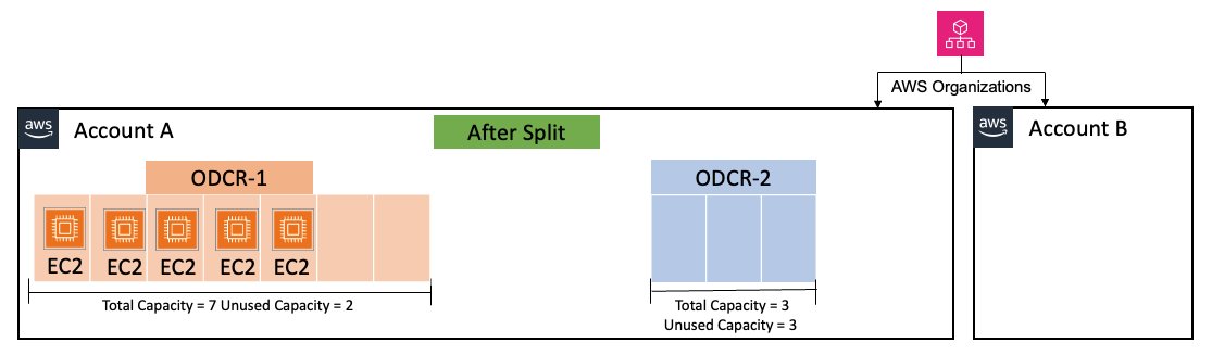
(Source: AWS News blog post)

The move capability allows users to transfer unused capacity slots between existing ODCRs. This optimizes resource utilization across different reservations, preventing wasted capacity and reducing costs. Users can reallocate resources to where they are needed most, improving overall efficiency.

The modify feature allows users to change reservation attributes without disrupting running workloads. Users can adjust the instance quantity, switch between targeted and open reservation types, and modify the reservation’s end date. This eliminates the need to create new reservations for minor adjustments and reduces operational overhead.

“These new capabilities provide you with powerful tools for improved capacity management and resource usage, leading to more efficient operations and cost savings,” states the AWS blog post, highlighting the benefits of these updates. The enhancements aim to improve capacity management, offering greater flexibility and control. By optimizing resource utilization and minimizing disruptions, users can achieve cost savings and improve the overall efficiency of their EC2 deployments.

The company writes in the blog post:

The ability to dynamically adjust and share Capacity Reservations provides the flexibility you need while maintaining the stability necessary for your critical workloads.

While cloud providers like Microsoft Azure and Google Cloud Platform (GCP) offer similar capacity reservation mechanisms, the specific features differ. Azure’s Reserved Virtual Machine Instances (Reserved VMs) and GCP’s Committed Use Discounts (CUDs) provide cost savings for committed compute usage. However, the newly introduced AWS “split, move, and modify” features offer more granular control over reservations than Azure and GCP’s standard offerings.

Article originally posted on InfoQ. Visit InfoQ

Transcript

Arik: I’ve called this, navigating LLM deployment: tips, tricks, and techniques 2.0. I could also rename it, how to deploy LLMs if you don’t work at Meta, OpenAI, Google, Mistral, or Anthropic. I’m specifically interested in how you deploy LLMs if you’re not serving it as a business, and instead you’re serving it so you can build applications on top of it, and you end up deploying it in fairly different ways if you work at a normal company versus one of these guys.

Hopefully you’re going to get three things out of this session. Firstly, you’re going to learn when self-hosting is right for you, because you’re going to find out it can be a bit of a pain, and it’s something you should only do if you really need to. Understanding the differences between your deployments and the deployments of AI Labs. Then, also, I’m going to give some best practices, tips, tricks, techniques, a non-exhaustive list for how to deploy AI in corporate and enterprise environments. Essentially, we build infrastructure for serving LLMs.

Evaluating When Self-Hosting is Right for You

Firstly, when should you self-host? To explain what that is, I’ll just clarify what I mean by self-hosting. I distinguish self-hosting compared to interacting with LLMs through an API provider. This is how you interact with LLMs through an API provider. They do all of the serving and hosting for you. It’s deployed on their GPUs, not your GPUs. They manage all of their infrastructure, and what they expose is just an API that you can interact with. That’s what an API hosted model is. All of those companies I mentioned at the beginning host these models for you. Versus being self-hosted. When you self-host, you’re in control of the GPUs. You take a model from Hugging Face or wherever you’re taking that model from, and you deploy it and you serve it to your end users. This is the broad difference. It’s essentially a matter of who owns the GPUs and who’s responsible for that serving infrastructure. Why would you ever want to self-host? Because when people manage things for you, your life is a little bit easier.

There are three main reasons why you’d want to self-host. The first one is you have decreased costs. You have decreased costs when you’re starting to scale. At the very early stages of POCing and trying things out, you don’t have decreased costs. It’s actually much cheaper to use an API provider where you pay per token, and the per token price is very low. Once you get to any kind of scale where you can fully utilize a GPU or close to it, it actually becomes much more cost efficient. The second reason why you’d want to self-host is improved performance. This might sound counterintuitive, because on all the leading benchmarks, the GPT models and the Claude models are best-in-class to those benchmarks.

However, if you know your domain and you know your particular use case, you can get much better performance when self-hosting. I’m going to talk about this a bit more later. This is especially true for embedding models, search models, reranker models. The state of the art for most of them is actually in open source, not in LLMs. If you want the best of the best breed models, you’ll have a combination of self-hosting for some models and using API providers for others. You can get much better performance by self-hosting. Some privacy and security. I’m from Europe, and we really care about this. We also work with regulated industries here in the U.S., where you have various reasons why you might want to deploy it within your own environment. Maybe you have a multi-cloud environment, or maybe you’re still on-prem. This sits with the data that a16z collected, that there’s broadly three reasons why people self-host: control, customizability, and cost. It is something that a lot of people are thinking about.

How do I know if I fall into one of those buckets? Broadly, if I care about decreased cost, that’s relevant to me if I’m deploying at scale, or it’s relevant to me if I’m able to use a smaller specialized model for my task run than a very big general model like GPT-4. If I care about performance, I will get improved performance if I’m running embedding or reranking workloads, or if I’m operating in a specialized domain that might benefit from fine-tuning. Or I have very clearly defined task requirements, I can often do better if I’m self-hosting, rather than using these very generic models.

Finally, on the privacy and security things, you might have legal restrictions, you’ll obviously then have to self-host. Potentially, you might have region-specific deployment requirements. We work with a couple clients who, because of the various AWS regions and Azure regions, they have to self-host to make sure they’re maintaining that sovereignty in their deployments. Then, finally, if you have multi-cloud or hybrid infrastructure, that’s normally a good sign that you need to self-host. A lot of people fall into those buckets, which is why the vast majority of enterprises are looking into building up some kind of self-hosting infrastructure, not necessarily for all of their use cases, but it’s good to have as a sovereignty play.

I’m going to make a quick detour. Quick public service announcement that I mentioned embedding models, and I mentioned that the state of the art for embedding models is actually in the open-source realm, or they’re very good. There’s another reason why you should almost always self-host your embedding models. The reason why is because you use your embedding models to create your vector database, and you’ve indexed vast amounts of data. If that embedding model that you’re using through an API provider ever goes down or ever is depreciated, you have to reindex your whole vector database. That is a massive pain. You shouldn’t do that. They’re very cheap to host as well. Always self-host your embedding models.

When should I self-host versus when should I not? I’ve been a little bit cheeky here. Good reasons to self-host. You’re building for scale. You’re deploying in your own environment. You’re using embedding models or reranker models. You have domain-specific use cases. Or my favorite one, you have trust issues. Someone hurt you in the past, and you want to be able to control your own infrastructure. That’s also a valid reason. Bad reasons to self-host is because you thought it was going to be easy. It’s not easier, necessarily, than using API providers. Or someone told you it was cool. It is cool, but that’s not a good reason. That is why. That’s how you should evaluate whether self-hosting is right for you. If you fall into one of these on the left, you should self-host. If not, you shouldn’t.

Understanding the Difference between your Deployments and Deployments at AI Labs

Understanding the difference between your deployments and the deployments in AI Labs. If I’m, for example, an OpenAI, and I’m serving these language models, I’m not just serving one use case. I’m serving literally millions of different use cases. That means I end up building my serving stack very differently. You, let’s say I’m hosting with an enterprise or corporate environment. Maybe I’m serving 20 use cases, like in a more mature enterprise. Maybe I’m serving now just a couple. Because I have that difference, I’m able to make different design decisions when it comes to my infrastructure. Here are a couple reasons why your self-hosting regime will be very different to the OpenAI self-hosting regime. First one is, they have lots of H100s and lots of cash.

The majority of you guys don’t have lots of H100s, and are probably renting them via AWS. They’re more likely to be compute bound because they’re using the GPUs like H100s, rather than things like A10s. They have very little information about your end workload, so they are just going on a, we’re just trying to stream tokens out for arbitrary workloads. You have a lot more information about your workload. They’re optimizing for one or two models, which means they can do things that just don’t scale for regular people, self-hosting. If I’m deploying just GPT-4, then I’m able to make very specific optimizations that only work for that model, which wouldn’t work anywhere else.

If you’re not self-hosting, you’re likely using cheaper, smaller GPUs. You’re probably using also a range of GPUs, so not just one type, maybe you’re using a couple different types. You want it to be memory bound, not compute bound. You have lots of information about your workload. This is something that is very exciting, that for most enterprises the workloads actually look similar, which is normally some kind of long-form RAG or maybe extraction task, and you can make decisions based on that. You’ll have to deal with dozens of model types, which is a luxury. You just don’t have the luxury of those AI Labs. Here are some differences between the serving that you’ll do, and the serving that your AI Labs will have to do.

Learning Best Practices for Self-Hosted AI Deployments in Corporate and Enterprise Environments

Best practices, there are literally an infinite number of best practices that I could give, but I’ve tried to boil them down to I think it’s now six non-exhaustive tips for self-hosting LLMs. This isn’t a complete guide to self-hosting, but hopefully there are some useful things that we’ve learned over the last couple years that might be useful to you. The first one is, know your deployment boundaries and work backwards. Quantized models are your friend. Getting batching right really matters. Optimize for your workload. That goes back to what I said earlier about, you can do optimizations that they just can’t. Be sensible about the models you use. Then, finally, consolidate infrastructure within your org. These are the top tips that I’m going to talk through now for the rest of the session.

1. Deployment Boundaries

Let’s start with deployment boundaries. Assuming you don’t have unlimited compute, and even AI Labs don’t have unlimited compute. It’s a really scarce resource at the moment. You need to be very aware of what your deployment requirements are, and then work backwards from what you know about them. If you know you only have a certain available hardware, maybe you’re, for example, just CPU bound, and you’re deploying completely on-prem, and you don’t have GPUs, then you probably shouldn’t be looking into deploying a Llama 4 billion or 5 billion. Knowing that boundary is important from the get go. You should have an idea of your target latency as well. You should have an idea of your expected load.

If you have all of these together, and you can construct some sentence of, I would like to deploy on an instance cheaper than x, which will serve y concurrent users in an average latency of less than z. If you can form that sentence, it makes everything else that you have to do much easier, and you won’t have that bottleneck of being like, “I built this great application. I just have no idea how to deploy it”. I can use that information to then work backwards and figure out what kind of models I should be looking at and how much effort I should be putting into things like prompting and really refining my search techniques, rather than upgrading to bigger models.

2. Quantize

Which leads me on to my second tip, which is, you should pretty much always be using quantized models, for a couple different reasons. The first reason I’m going to say is that you should always use quantized models, more or less, is because the accuracy is pretty much always better than a model of that same memory requirement that you’ve quantized it down to, so you retain a lot of that accuracy. The second reason that you should pretty much always quantize is actually the accuracy loss isn’t that different from the original model. I’ll reference two pieces of research that show this. There was this paper that came out in 2023, by Tim Dettmers, amongst others, who’s a bit of a legend in the field, and it’s called, “The case for 4-bit precision”. What he showed in this paper, actually, the highlight figure, is that for a fixed model bit size, the accuracy of the model is far higher if you’re using a quantized model.

Given that we know when we have a model with more parameters, as I scale up the parameters, the accuracy of the model goes up. What’s interesting is, if I take one of those large models and quantize it down to a natively smaller size, it retains a lot of that accuracy that we had in the beginning, which is very good. I’m pretty much always going to have better performance using a quantized 70 billion parameter model than I will of a model of a native size. This goes on to some great research that Neural Magic did on this. They showed that, firstly, if I quantize models, so here they have the accuracy recovery. This is when they take original bit precision models and then quantize them. It pretty much retains all of the accuracy from the original model, which is great. You get like 99% accuracy maintenance, which is awesome. You can see that even though there are slight dips in the performance, so, for example, if I look at this 405 here, with one of the quantized variants, it’s a slight dip in the original, like a couple of basis points.

It’s still far higher than the 70 billion parameter or the 8 billion parameter model. It retains much of that accuracy that you were looking for. If you know your deployment boundaries, and you don’t have unlimited amounts of compute to call from, using that quantized model, using the best model that will fit within that is a great piece of advice. If I know that this is the piece of infrastructure I’m working with, this is the GPU I’m working with, I can then say, ok, which is the biggest model that when quantized down to 4-bit, is going to perform the best?

In this case, at least a couple months old. Mixtral is not really a thing anymore, but you get the idea that I would rather use the Mixtral 4-bit, which is 22-gig, than the Llama 13B, because it’s retained a lot of that performance. I put at the bottom places that you can find quantized models. We retain an open-source bank of quantized models that you can check out. TheBloke also used to be a great source of this as well, although he’s not doing it as much recently.

3. Batching Strategies

The third thing I’m going to talk about is batching strategies. This is something that’s very important to get right. The reason it’s very important to get right is because it’s a very easy way to waste GPU resources. When you’re first deploying, you’re probably not using any batching, which means you end up with GPU utilization coming like this. It’s not great. We then see people going straight to dynamic batching. What this means is I have a set batch size, so let’s say my batch size is 16. I will wait until 16 requests have come in to process, or I’ll wait a fixed amount of time, and you end up with this spiky GPU utilization, which is still not great either. What’s far better if you’re deploying generative models, a very big piece of advice is to use something like continuous batching, where you can get consistently high GPU utilization.

It’s a state-of-the-art technique designed for batching of generative models, and it allows requests to interrupt long in-flight requests. This batching happens at the token level rather than happening at the request level. I could, for example, have my model generate the 65th token of one response, and then the fifth token of another response, and I end up with a utilization that is far more even. This is just one of the examples of inference optimizations that you can do that make a really big difference. Here, I think I’ve gone from a 10% utilization to near enough 80. Really significant improvements. If you’re in a regime where you don’t have much compute resource, this is a very valuable thing to do.

4. Workload Optimizations

I’m going to talk about workload optimizations. It’s something that we’ve been researching a lot actively, and we think is really promising. You know something that the AI Labs don’t know, which is you know what your workload looks like. What that means is you can make a lot of decisions based on what your workload looks like, that it would just never, ever make sense for them to make. I’m going to give you a couple examples of techniques that you can use that make sense if you know what your workload looks like, that don’t make sense if you’re serving big multi-tenant environments and multiple user groups. One of them is prefix caching. This is probably one of the things that I’m most excited by that happened this year.

One of the most common use cases that we see from our clients is situations where they have really long prompts, and often these prompts are shared between requests. Maybe what I have is I have a very long context RAG on a set document that maybe I just pass through the whole document and I’m asking questions of it. Or maybe I have a situation where I have a very long set of user instructions to the LLM. These are instances where I have very long prompts. Traditionally, what I would have to do is I’d have to reprocess that prompt every single request, which is super inefficient. What we can do, if you know what your workload looks like, and you know that you’re in a regime where you have a lot of shared prompts, or very long shared prompts, you can use something called prefix caching, which is essentially when you pre-compute the KV cache of text and you reuse that when the context is reused, when you do your next generation.

My LLM doesn’t need to reprocess that long prompt every single time, they can process just the difference between them. If I have a very long-shared prompt and then slightly different things each time, it can just process that difference and then return. On the right, I have some results that are fresh off the press. What we have here is our server with the prefix caching turned on and turned off. In the green lines, we have it turned off. The light green line is with two GPUs, and the dark green line is with one GPU. With the blue line, we have it with the prefix caching turned on. What you can see is we have very significant throughput improvement. It’s throughput on the Y and then batch size on the X. About 7x higher throughput, which is very significant. It means that you can process many more requests, or you can process those requests much cheaper.

This has like no impact, if you didn’t know that you had a long-shared prompt. It doesn’t really have an impact if I’m serving multiple dozens of users at any one time. This only really works if I know what my use case looks like. Another example of caching that we are really excited by. We call this internally, SSD, which is a form of speculative decoding, but you can also think of it like caching, which only makes sense if you know what your workload looks like. This is a use case where, if your model might predict similar tokens between tasks. Let’s say I’m doing a task where I have phrases that are very frequently repeated, what I can do is I can essentially cache those very frequently repeated phrases.

Instead of computing the whole phrase every single time, token by token, I can just pull a cache hit and inference on that. We did benchmarking on this, and for a workload of the JSON extractive workload, we got about a 2.5 latency decrease on this, which is pretty significant. Again, would have literally no impact if I’m using the OpenAI API, because there’s no way they could cache your responses, and 75 million other people’s responses. It only really makes sense if you’re deploying in your own environment.

5. Model Selection

I have two more that I’m going to go through. This one is model selection. I think everyone knows this by now, but the only real reason I put it up is because last time people really liked the image. This is something that I still see people getting wrong, which is, they get their large language models, which are the most difficult things to deploy and the most expensive things to deploy, to do pretty much all of the workload. That’s not a good idea. The reason it’s not a good idea is because you then have more of this difficult, expensive thing to manage. There are a lot of parts to an enterprise RAG pipeline. In fact, the most important part of your enterprise RAG pipeline is actually not the LLM at all. The most important part is your embedding and retrieval part, by far. They don’t need GPT-4 level reasoning, obviously.

If you have really good search and retrieval pipelines, you can actually use much smaller models to get the same results. We’ve seen clients move from GPT-4 type setups to move to things as small as the Llama 2 billion models, if they get their retrieval part right, which means you can run the whole application very cheaply. I would advise people to check out the Gemma and the small Llama models for this. We think they’re very good. Very good in extractive workloads as well, especially if you’re using a JSON structured format like Outlines or LMFE. Pick your application design carefully and only use big models when you really need to use big models.

6. Infrastructure Consolidation

Finally, I’m going to talk about infrastructure consolidation. In traditional ML, most teams actually work in silos still, unfortunately, which is, they deploy their own model and they’re responsible for deploying their own model. In GenAI, it does not make sense to do that, and that’s why these API providers are making an absolute killing, because it does make sense to deploy once, manage centrally, and then provide it as a shared resource within the organization. If you do this, it enables your end developers to focus on building this application level rather than building infrastructure. When I speak to my clients, sometimes we talk about building an internal version of the OpenAI API. That’s the experience you want to be able to provide to your developers, because otherwise they’ll have to learn what prefix caching is every single time they want to deploy a model, which is just not an efficient use of time.

I think this kind of centralization is a really exciting opportunity for MLOps teams to take that ownership within the org. This still means you can understand the kind of workloads you work with and optimize for, for example, long context RAG situations. That’s still something that you can do. You can actually end up making a cheaper and better version of something like the OpenAI API. Serving is hard. Don’t do it twice or even three. We’ve seen clients who do it over and again. You’ll have a team deploying with Ollama, another team deploying with vLLM, and trying to do it. Much better to have a central team manage that. GPUs are very expensive, don’t waste them.

I can talk about what this would actually look like in practice. This central consolidation of infrastructure, you can think of it as having like an internal Bedrock, or an internal OpenAI API, or something like that. Individual ML teams can work from these APIs and then build applications on top of them using techniques like LoRA, so that’s a form of fine-tuning, or they use things like RAG, where they’re plugging into it in the same way they use the OpenAI API. We have a quick case study, so a client of ours did this. They started off with a bunch of different models. Each app was essentially attached to its own model and attached to its own GPU setup. This is obviously not ideal, because I’m deploying, for example, at the time, it was a Mixtral. We were deploying that multiple times, over and again and wasting GPU resources.

Instead, what we did is we just pooled it into one and deployed that Mixtral on a centrally hosted infrastructure, which meant we could use much less GPU resource than we were using otherwise. Something that I like the pattern of, if you’re doing this central deployment and central hosting, is give your team access to a couple different models of different sizes, give them optionality. Don’t say something like, you can only use this particular model, because they want to be able to try things. Deploying a large, medium, and small model that you guys have checked out and that you’re happy with is a really good place to start with a bunch of maybe those auxiliary models, so table parses, embedding models, reranker models. If you do that, you give your team optionality, and you still maintain the benefit of being able to consolidate that infrastructure and make those optimizations.

There’s my six non-exhaustive tips for self-hosting LLMs. Know your deployment boundaries and work backwards. If you do know this, everything else becomes much easier. Quantized models are your friends. They might seem scary because they affect the model, but they’re actually, on the whole, much better. Getting batching right really matters for your GPU utilization. Optimize for your particular workload. You have a superpower that the API providers do not, which is, you know what your workload will look like. Be sensible about the models you use. Then, finally, consolidate infrastructure within your organization.

Summary

We’ve gone through, why you should self-host. There’s a bunch of infrastructural reasons why self-hosting is a great idea, for deploying at scale. If you want to use embedding models, reranker models, if you, for example, are using domain-specific models, all very good reasons to self-host. Your needs in deploying will be different to the needs of AI Labs and mass AI API providers, because you’re using different types of hardware and your workloads are different. I’ve also given six tips, best practices that we’ve learned over the last couple years for deploying LLMs in this kind of environment.

Questions and Answers

Luu: For those tips that you gave, if I have a bursty workload, are any of those tips more relevant than others?

Arik: If you have a bursty workload, it’s rough. Because there’s always going to be some cold start problem when you’re deploying these. For bursty workloads, they’re slightly less well suited for self-hosting, unless you’re deploying smaller models. If you’re deploying smaller models, the scaling up and scaling down is much easier, but if you’re deploying bigger models, consider whether you do need to actually self-host, or whether you can use other providers. We, within our infrastructure, have obviously built Kubernetes resources that can do that scaling up and scaling down.

If you have bursty workloads with very low latency requirements, that is just challenging. What you could do, and what we have seen people do is, if they have a bursty workload, migrating to smaller and cheaper models during the periods of high burst and then going back to the higher performance models when things are a bit more chill. You could imagine a regime where you had a 70 billion parameter model servicing most of the requests, and then let’s say you get to periods of very high load, while you’re waiting to scale up, you move to something like an 8 billion parameter model or something slightly smaller. You take a small accuracy hit, and then go from there. That’s something that we’ve seen work as well.

Participant 1: How would you architect a central compute infra, if each downstream application requires different fine-tuning, where you can’t really have an internal OpenAI API like serving infrastructure?

Arik: That’s very difficult if you want to do something like full fine-tuning, which we’ve been used to over the last couple years, which essentially you fine-tune the whole model. Because what that means is, every single time you fine-tune the model, you have to deploy a separate instance of it. Fortunately, over the last two years, there’s been advancements in PEFT methods, which is essentially a way that you can fine-tune, but you don’t have to fine-tune the whole model. You can just fine-tune a small subsection of it. Let’s say I have a situation where I’m centrally hosting and I have 10 different teams, and every single team has done a fine-tuned version of a Llama model, for example. What I used to have to do is go in and deploy each of those on their own GPUs or shared GPUs. What I can do now instead is just deploy a centrally hosted Llama model, and then deploy on the same GPU still, in my same server, all of these different LoRA fine-tuned versions. These small adapters that we add to all of the models.

On inference time, we can hot swap them in and out. It’s like you’re calling separate models, but actually it’s one base model and these different adapters. That’s really exciting, because it means we can deploy hundreds if not thousands of fine-tuned, domain-specific models with the exact same infrastructure and resource that we need to deploy one. That’s the way I would go about it, PEFT methods. We prefer LoRA as a method, but there are other available on the market.

Participant 2: You’re speaking a lot about the models themselves, which is awesome, but in your diagrams, when you’re referring to GPUs, and all the work that you did, should we assume most of this is based on HB100 Blackwell, NVIDIA, or did you actually go across Gaudi and Instinct from AMD and so on? Just curious, because we’re looking to build something. Support for all models is not ubiquitous right now. Where did you stop and start with how far your suggestions go here, on some of that hardware level?

Arik: We very rarely see clients deploying on like H100 or B100s. The kinds of clients that we work with are enterprise and corporates, which might have access to the previous generations of GPUs or maybe slightly cheaper GPUs. We tend to do most of our benchmarking on those kinds of GPUs. We support NVIDIA and AMD. We’re rolling out support for Intel as well. We have seen good results on AMD. We think they’re a really interesting option. Then for Intel, we’re waiting for the software support to catch up there. We also know that like Inferentia are doing interesting things, and the TPUs are doing interesting things as well. There’s definitely more out there than the B100s and H100s that you see.

For most enterprises, you really don’t need them, and that you’ll probably find with previous generations of NVIDIA hardware. My recommendation would be to stick with NVIDIA, mainly because the software stack is a bit more evolved. I would build your infrastructure and applications such that you can move to AMD or you can move to other providers in a couple years, because that gap is going to close pretty quickly, so you don’t want to tie yourself to like an NVIDIA native everything.

Participant 2: We’re using OpenAI off of Azure, so we’re using NVIDIA, but I’m looking to build something out locally, because we’ll balance loads between cloud and on-prem for development, or even just spilling over extra load. Keeping mind open to everything.

Arik: One of our selling points is that we are hardware agnostic, so we can deploy on not just NVIDIA, but others as well. The conversation always goes something like, can I deploy on AMD? We’re like, yes. Do you use AMD? No, but I might want to. It’s a good thing to keep your options open there.

Participant 3: Could you elaborate on some of the batching techniques?

Arik: Let’s assume we’re not going to do no batching, and we’re going to do some kind of batching. If I’m doing dynamic batching, what’s happening is this is batching on a request level. Let’s say my batch size is 16. I’m going to wait for 16 requests to come in, and then I’m going to process them. If I’m in a period of very low traffic, I’ll also have some time as well, so maybe either 16 or a couple seconds, and then I’ll process that batch. What that means is I get this spiky workload where I’m waiting for long requests to finish and stuff like that. What we can do instead is this continuous batching. What this allows you to do is it allows you to interrupt very long responses with other responses as well. This means that we can do essentially like token level processing rather than request level.

I might have a situation where I have a very long response, and I can interrupt that response every so often to process shorter responses as well. It means that my GPU is always at very high utilization, because I’m constantly feeding it new things to do. We end up with continuous batching, which is much better GPU utilization.

Luu: Just token level.

Participant 4: How does interrupting and giving it a different task improve GPU utilization? Why not just continue with the current task, gives you the peak utilization at all times.

Arik: Essentially, it’s because otherwise you have to wait for that whole request to finish, and the GPU is able to process things in parallel, so it doesn’t actually affect the quality of the output at all. It just means that each pass, I can just have it predict different tokens from different requests. It’s constantly being fed with new things, rather than waiting for the longest response to finish, and it’s only working on that one response while we’re waiting for a new batch.

Participant 4: You’re suggesting I can put multiple requests in at the same time, in a single request to the GPU.

Arik: Exactly. What you end up with is your latency, on average, is a little bit higher, but my throughput is much better. If I batch these requests together and process them together, I end up getting much better throughput than if I was just to process them one by one.

Participant 4: When I do give it a long-running request, what is GPU doing if it’s not being utilized 100% percent? What is taking that long? Why is the request taking that long while GPU is not being utilized? What is going on in that setup?

Arik: When the GPU is not being utilized?

Participant 4: Yes. You’re saying, I’m putting in a long-running request, so it is running. What is running if the GPU is not being utilized at the same time to maximum capacity?

Arik: It’s essentially doing each request one by one, so I have to wait until the next one. I have a fairly good article, I think Baseten wrote, which also was very good in this.

See more presentations with transcripts