Category: Uncategorized

MMS • RSS
![]() MongoDB, Inc. (NASDAQ:MDB – Get Free Report) was the recipient of unusually large options trading activity on Wednesday. Stock investors acquired 36,130 call options on the company. This represents an increase of 2,077% compared to the average daily volume of 1,660 call options.
MongoDB, Inc. (NASDAQ:MDB – Get Free Report) was the recipient of unusually large options trading activity on Wednesday. Stock investors acquired 36,130 call options on the company. This represents an increase of 2,077% compared to the average daily volume of 1,660 call options.
MongoDB Trading Up 1.8%
Shares of MongoDB stock opened at $228.25 on Thursday. The business has a 50-day moving average price of $204.58 and a two-hundred day moving average price of $212.84. MongoDB has a 1-year low of $140.78 and a 1-year high of $370.00. The company has a market cap of $18.65 billion, a P/E ratio of -200.22 and a beta of 1.41.
MongoDB (NASDAQ:MDB – Get Free Report) last released its quarterly earnings data on Wednesday, June 4th. The company reported $1.00 earnings per share (EPS) for the quarter, topping analysts’ consensus estimates of $0.65 by $0.35. The company had revenue of $549.01 million for the quarter, compared to analysts’ expectations of $527.49 million. MongoDB had a negative net margin of 4.09% and a negative return on equity of 3.16%. The business’s revenue was up 21.8% on a year-over-year basis. During the same quarter in the prior year, the firm earned $0.51 EPS. Equities research analysts forecast that MongoDB will post -1.78 EPS for the current fiscal year.
Insider Buying and Selling
<!—->
In other MongoDB news, Director Dwight A. Merriman sold 820 shares of the business’s stock in a transaction dated Wednesday, June 25th. The shares were sold at an average price of $210.84, for a total value of $172,888.80. Following the completion of the transaction, the director directly owned 1,106,186 shares of the company’s stock, valued at approximately $233,228,256.24. The trade was a 0.07% decrease in their ownership of the stock. The sale was disclosed in a legal filing with the SEC, which is accessible through this hyperlink. Also, CEO Dev Ittycheria sold 3,747 shares of the firm’s stock in a transaction dated Wednesday, July 2nd. The stock was sold at an average price of $206.05, for a total value of $772,069.35. Following the sale, the chief executive officer directly owned 253,227 shares in the company, valued at approximately $52,177,423.35. This represents a 1.46% decrease in their position. The disclosure for this sale can be found here. Over the last ninety days, insiders sold 32,746 shares of company stock worth $7,500,196. Corporate insiders own 3.10% of the company’s stock.
Hedge Funds Weigh In On MongoDB
Several large investors have recently added to or reduced their stakes in MDB. Jericho Capital Asset Management L.P. bought a new position in shares of MongoDB during the 1st quarter worth approximately $161,543,000. Norges Bank purchased a new position in MongoDB in the fourth quarter valued at about $189,584,000. Primecap Management Co. CA boosted its stake in MongoDB by 863.5% in the first quarter. Primecap Management Co. CA now owns 870,550 shares of the company’s stock valued at $152,694,000 after acquiring an additional 780,200 shares during the last quarter. Westfield Capital Management Co. LP bought a new stake in shares of MongoDB in the 1st quarter worth approximately $128,706,000. Finally, Vanguard Group Inc. raised its holdings in shares of MongoDB by 6.6% in the 1st quarter. Vanguard Group Inc. now owns 7,809,768 shares of the company’s stock worth $1,369,833,000 after purchasing an additional 481,023 shares during the period. Institutional investors own 89.29% of the company’s stock.
Analyst Ratings Changes
A number of analysts recently weighed in on MDB shares. William Blair reaffirmed an “outperform” rating on shares of MongoDB in a report on Thursday, June 26th. Bank of America raised their price objective on shares of MongoDB from $215.00 to $275.00 and gave the company a “buy” rating in a research note on Thursday, June 5th. Stifel Nicolaus dropped their price target on shares of MongoDB from $340.00 to $275.00 and set a “buy” rating on the stock in a report on Friday, April 11th. Monness Crespi & Hardt raised shares of MongoDB from a “neutral” rating to a “buy” rating and set a $295.00 price objective on the stock in a report on Thursday, June 5th. Finally, Stephens assumed coverage on shares of MongoDB in a report on Friday, July 18th. They issued an “equal weight” rating and a $247.00 price objective on the stock. Nine research analysts have rated the stock with a hold rating, twenty-six have given a buy rating and one has issued a strong buy rating to the company’s stock. Based on data from MarketBeat, MongoDB has a consensus rating of “Moderate Buy” and an average target price of $281.35.
Read Our Latest Analysis on MongoDB
MongoDB Company Profile
MongoDB, Inc, together with its subsidiaries, provides general purpose database platform worldwide. The company provides MongoDB Atlas, a hosted multi-cloud database-as-a-service solution; MongoDB Enterprise Advanced, a commercial database server for enterprise customers to run in the cloud, on-premises, or in a hybrid environment; and Community Server, a free-to-download version of its database, which includes the functionality that developers need to get started with MongoDB.
Featured Stories
Receive News & Ratings for MongoDB Daily – Enter your email address below to receive a concise daily summary of the latest news and analysts’ ratings for MongoDB and related companies with MarketBeat.com’s FREE daily email newsletter.
ExaGrid 7.3.0 Expands Backup Support, Now Covering Rubrik, MongoDB, and Microsoft SQL Server
MMS • RSS
ExaGrid, the industry’s only Tiered Backup Storage solution with Retention Time-Lock that includes a non-network-facing tier (creating a tiered air gap), delayed deletes, and immutability for ransomware recovery, is debuting ExaGrid software version 7.3.0, ushering in support for industry-leading backup applications and utilities.
ExaGrid Tiered Backup Storage offers fast backups, fast recoveries, and comprehensive security, underscored by a cost-efficient, scale-out architecture, according to the vendor.. Easy to install and use, ExaGrid works with over 25 backup applications, enabling backups from multiple backup apps simultaneously. With version 7.3.0, ExaGrid continues this momentum with the following support:
- Rubrik backup software using the Rubrik Archive Tier or Rubrik Archive Tier with Instant Archive enabled
- MongoDB Ops Manager, the powerful management tool designed for organizations using MongoDB at scale
- Deduplication for encrypted Microsoft SQL Server direct dumps, where when encryption is enabled in the SQL application (TDE), ExaGrid can achieve about a 4:1 data reduction via ExaGrid’s advanced Adaptive Data Deduplication technology
“ExaGrid continues to add and improve on our integrations with the industry’s leading backup applications and utilities. We are excited to expand our list of supported backup applications to include Rubrik and MongoDB,” said Bill Andrews, president and CEO of ExaGrid. “We are also pleased to offer storage and cost savings for SQL database dumps that are encrypted by TDE. ExaGrid remains committed to offering a solution that solves all the challenges of backup storage, and we look forward to adding value for current and future customers with the release of Version 7.3.0.”
To learn more about ExaGrid 7.3.0, please visit https://www.exagrid.com/.
MMS • RSS
MongoDB (MDB, Financial) is witnessing a notable increase in bullish option activity, with 9,882 call options traded, which is 1.7 times the usual volume. This surge comes alongside a rise in implied volatility, now at 48.23%. The most heavily traded options are the weekly calls at the $235 strike for July 25 and the January 2026 calls at the $250 strike, collectively amounting to nearly 2,100 contracts.
The current Put/Call Ratio stands at 0.59, indicating a preference toward call options. Investors are keeping a close watch as the company’s earnings announcement is anticipated on August 28.
Wall Street Analysts Forecast
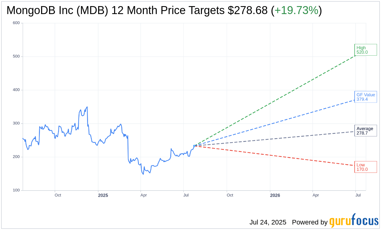
Based on the one-year price targets offered by 38 analysts, the average target price for MongoDB Inc (MDB, Financial) is $278.68 with a high estimate of $520.00 and a low estimate of $170.00. The average target implies an
upside of 19.73%
from the current price of $232.75. More detailed estimate data can be found on the MongoDB Inc (MDB) Forecast page.
Based on the consensus recommendation from 39 brokerage firms, MongoDB Inc’s (MDB, Financial) average brokerage recommendation is currently 1.9, indicating “Outperform” status. The rating scale ranges from 1 to 5, where 1 signifies Strong Buy, and 5 denotes Sell.
Based on GuruFocus estimates, the estimated GF Value for MongoDB Inc (MDB, Financial) in one year is $379.42, suggesting a
upside
of 63.02% from the current price of $232.75. GF Value is GuruFocus’ estimate of the fair value that the stock should be traded at. It is calculated based on the historical multiples the stock has traded at previously, as well as past business growth and the future estimates of the business’ performance. More detailed data can be found on the MongoDB Inc (MDB) Summary page.
MDB Key Business Developments
Release Date: June 04, 2025
- Revenue: $549 million, a 22% year-over-year increase.
- Atlas Revenue: Grew 26% year over year, representing 72% of total revenue.
- Non-GAAP Operating Income: $87 million, with a 16% non-GAAP operating margin.
- Customer Count: Over 57,100 customers, with approximately 2,600 added sequentially.
- Net ARR Expansion Rate: Approximately 119%.
- Gross Margin: 74%, down from 75% in the year-ago period.
- Net Income: $86 million or $1 per share.
- Operating Cash Flow: $110 million.
- Free Cash Flow: $106 million.
- Cash and Equivalents: $2.5 billion.
- Share Repurchase Program: Increased by $800 million, totaling $1 billion.
- Q2 Revenue Guidance: $548 million to $553 million.
- Fiscal Year ’26 Revenue Guidance: $2.25 billion to $2.29 billion.
- Fiscal Year ’26 Non-GAAP Income from Operations Guidance: $267 million to $287 million.
For the complete transcript of the earnings call, please refer to the full earnings call transcript.
Positive Points
- MongoDB Inc (MDB, Financial) reported a 22% year-over-year increase in revenue, reaching $549 million, surpassing the high end of their guidance.
- Atlas revenue grew 26% year over year, now representing 72% of total revenue, indicating strong adoption of their cloud-based platform.
- The company achieved a non-GAAP operating income of $87 million, resulting in a 16% non-GAAP operating margin, which is an improvement from the previous year.
- MongoDB Inc (MDB) added approximately 2,600 new customers in the quarter, bringing the total customer count to over 57,100, the highest net additions in over six years.
- The company announced a significant expansion of their share repurchase program, authorizing up to an additional $800 million, reflecting confidence in their long-term potential.
Negative Points
- Despite strong results, MongoDB Inc (MDB) noted some softness in Atlas consumption in April due to macroeconomic volatility, although it rebounded in May.
- The non-Atlas business is expected to decline in the high single digits for the year, with a $50 million headwind from multiyear license revenue anticipated in the second half.
- Gross margin slightly declined to 74% from 75% in the previous year, primarily due to Atlas growing as a percentage of the overall business and the impact of the Voyage acquisition.
- The company experienced slower than planned headcount additions, which could impact future growth and operational capacity.
- MongoDB Inc (MDB) remains cautious about the uncertain macroeconomic environment, which could affect future consumption trends and overall business performance.
.NET 10 Preview 6 Introduces Blazor Enhancements, Memory Optimization, and SDK Improvements
MMS • Almir Vuk
Microsoft has announced the sixth preview of .NET 10, introducing a broad range of enhancements across the .NET Runtime, SDK, libraries, C#, ASP.NET Core, Blazor, and .NET MAUI. As stated in the official release, the update focuses on improving performance, developer experience, and cross-platform tooling.
In the realm of ASP.NET Core, memory management has been refined. Kestrel, IIS, and HTTP.sys now supports automatic eviction of unused memory from its internal pools when applications are idle. As reported, this change requires no developer action and is designed to reduce memory usage efficiently. Metrics for memory pools are now exposed under Microsoft.AspNetCore.MemoryPool, and developers can build custom memory pools using the new IMemoryPoolFactory interface.
Blazor also receives several key updates. A new component offers more control over preloading framework assets, improving performance and base URL detection. Blazor WebAssembly projects can now generate output compatible with JavaScript bundlers like webpack by setting WasmBundlerFriendlyBootConfig to true, allowing, as stated, better integration with modern frontend pipelines.
Validation support in Blazor has been extended to include nested objects and collections within forms. This new capability is enabled through AddValidation() and the [ValidatableType] attribute. With a note that the attribute remains experimental and requires diagnostic suppression. Blazor diagnostics were improved as well, with traces for server circuits now exposed as top-level activities, simplifying telemetry in tools like Application Insights.
Blazor Server now supports persisting circuit state, allowing users to resume activity after reconnecting, even after server-side eviction. Developers can control circuit behavior through the new Blazor.pause() and Blazor.resume() APIs, as explained this will help reduce server resource consumption during idle periods.
Navigation behavior in Blazor was updated for consistency, with a configuration switch now opt-in to disable NavigationException usage. ASP.NET Core Identity now includes support for passkeys, enabling modern, phishing-resistant authentication using the WebAuthn and FIDO2 standards. The Blazor Web App template includes built-in support for this.
Minimal APIs can now integrate validation error responses using IProblemDetailsService, offering more consistent and customizable error output. As reported, the validation APIs have moved to a new Microsoft.Extensions.Validation package and namespace, broadening their usage beyond ASP.NET Core.
Regarding the .NET MAUI, the MediaPicker component was enhanced to support multiple file selection and in-API image compression. Developers can also now intercept web requests within BlazorWebView and HybridWebView, enabling advanced scenarios like modifying headers or injecting custom responses.
Furthermore, various UI fixes were implemented across controls, including CollectionView, CarouselView, and SearchBar, along with memory leak resolutions and improved rendering on Windows, Android, and iOS. Additionally, .NET now supports Android API levels 35 and 36, and includes diagnostics and interop performance improvements. On Apple platforms, the release aligns with Xcode 16.4 and brings reliability and runtime enhancements.
The .NET SDK introduces major improvements for tool authors, including support for platform-specific tools within a single package, and the new dotnet tool exec command, which, as described in the official docs, allows one-shot execution without installation. Also the lightweight dnx script further simplifies tool execution.
CLI introspection capabilities were extended with the –cli-schema option, which outputs a machine-readable JSON representation of commands, aiding automation and scripting. File-based apps received additional improvements, including support for native AOT publishing, project references, and enhanced shebang support for shell execution.
For interested readers, full release notes and further technical documentation are available on the official .NET documentation, also the developers can join the GitHub discussion.
MMS • RSS

Investors in MongoDB, Inc MDB need to pay close attention to the stock based on moves in the options market lately. That is because the Aug 15, 2025 $350 Put had some of the highest implied volatility of all equity options today.
What is Implied Volatility?
Implied volatility shows how much movement the market is expecting in the future. Options with high levels of implied volatility suggest that investors in the underlying stocks are expecting a big move in one direction or the other. It could also mean there is an event coming up soon that may cause a big rally or a huge sell-off. However, implied volatility is only one piece of the puzzle when putting together an options trading strategy.
What do the Analysts Think?
Clearly, options traders are pricing in a big move for MongoDB shares, but what is the fundamental picture for the company? Currently, MongoDB is a Zacks Rank #2 (Buy) in the Internet – Software industry that ranks in the Top 30% of our Zacks Industry Rank. Over the last 60 days, seven analysts have increased their earnings estimates for the current quarter, while one analyst has revised the estimate downward. The net effect has taken our Zacks Consensus Estimate for the current quarter from 59 cents per share to 64 cents in that period.
Given the way analysts feel about MongoDB right now, this huge implied volatility could mean there’s a trade developing. Oftentimes, options traders look for options with high levels of implied volatility to sell premium. This is a strategy many seasoned traders use because it captures decay. At expiration, the hope for these traders is that the underlying stock does not move as much as originally expected.
Looking to Trade Options?
Check out the simple yet high-powered approach that Zacks Executive VP Kevin Matras has used to close recent double and triple-digit winners. In addition to impressive profit potential, these trades can actually reduce your risk.
Click to see the trades now >>
This article originally published on Zacks Investment Research (zacks.com).
Zacks Investment Research
MMS • RSS
![]() Cwm LLC raised its stake in MongoDB, Inc. (NASDAQ:MDB – Free Report) by 8.7% during the 1st quarter, according to its most recent Form 13F filing with the Securities and Exchange Commission. The firm owned 3,607 shares of the company’s stock after buying an additional 289 shares during the quarter. Cwm LLC’s holdings in MongoDB were worth $633,000 as of its most recent filing with the Securities and Exchange Commission.
Cwm LLC raised its stake in MongoDB, Inc. (NASDAQ:MDB – Free Report) by 8.7% during the 1st quarter, according to its most recent Form 13F filing with the Securities and Exchange Commission. The firm owned 3,607 shares of the company’s stock after buying an additional 289 shares during the quarter. Cwm LLC’s holdings in MongoDB were worth $633,000 as of its most recent filing with the Securities and Exchange Commission.
Several other hedge funds have also recently added to or reduced their stakes in the stock. 111 Capital bought a new stake in shares of MongoDB in the 4th quarter valued at about $390,000. Park Avenue Securities LLC grew its holdings in MongoDB by 52.6% during the first quarter. Park Avenue Securities LLC now owns 2,630 shares of the company’s stock valued at $461,000 after purchasing an additional 907 shares during the period. Cambridge Investment Research Advisors Inc. grew its holdings in MongoDB by 4.0% during the first quarter. Cambridge Investment Research Advisors Inc. now owns 7,748 shares of the company’s stock valued at $1,359,000 after purchasing an additional 298 shares during the period. Sowell Financial Services LLC bought a new position in shares of MongoDB during the first quarter worth $263,000. Finally, Farther Finance Advisors LLC boosted its position in shares of MongoDB by 57.2% during the first quarter. Farther Finance Advisors LLC now owns 1,242 shares of the company’s stock worth $219,000 after purchasing an additional 452 shares in the last quarter. Institutional investors and hedge funds own 89.29% of the company’s stock.
Analysts Set New Price Targets
A number of equities analysts have recently weighed in on the stock. Daiwa America raised shares of MongoDB to a “strong-buy” rating in a research report on Tuesday, April 1st. Needham & Company LLC reissued a “buy” rating and set a $270.00 price target on shares of MongoDB in a research report on Thursday, June 5th. Truist Financial reduced their price target on shares of MongoDB from $300.00 to $275.00 and set a “buy” rating on the stock in a research report on Monday, March 31st. Scotiabank lifted their price target on shares of MongoDB from $160.00 to $230.00 and gave the stock a “sector perform” rating in a research report on Thursday, June 5th. Finally, Royal Bank Of Canada reissued an “outperform” rating and set a $320.00 price target on shares of MongoDB in a research report on Thursday, June 5th. Nine research analysts have rated the stock with a hold rating, twenty-six have issued a buy rating and one has issued a strong buy rating to the stock. Based on data from MarketBeat, the company currently has an average rating of “Moderate Buy” and a consensus target price of $281.35.
<!—->
Get Our Latest Stock Report on MDB
MongoDB Price Performance
MongoDB stock opened at $228.25 on Thursday. The company’s 50-day moving average is $204.58 and its 200-day moving average is $212.84. The firm has a market capitalization of $18.65 billion, a PE ratio of -200.22 and a beta of 1.41. MongoDB, Inc. has a fifty-two week low of $140.78 and a fifty-two week high of $370.00.
MongoDB (NASDAQ:MDB – Get Free Report) last posted its quarterly earnings results on Wednesday, June 4th. The company reported $1.00 EPS for the quarter, topping analysts’ consensus estimates of $0.65 by $0.35. MongoDB had a negative return on equity of 3.16% and a negative net margin of 4.09%. The business had revenue of $549.01 million during the quarter, compared to analysts’ expectations of $527.49 million. During the same quarter last year, the company posted $0.51 earnings per share. MongoDB’s quarterly revenue was up 21.8% on a year-over-year basis. As a group, analysts expect that MongoDB, Inc. will post -1.78 EPS for the current year.
Insider Buying and Selling
In related news, CEO Dev Ittycheria sold 25,005 shares of MongoDB stock in a transaction dated Thursday, June 5th. The shares were sold at an average price of $234.00, for a total transaction of $5,851,170.00. Following the completion of the sale, the chief executive officer owned 256,974 shares of the company’s stock, valued at approximately $60,131,916. The trade was a 8.87% decrease in their position. The sale was disclosed in a filing with the SEC, which is accessible through the SEC website. Also, Director Dwight A. Merriman sold 2,000 shares of MongoDB stock in a transaction dated Thursday, June 5th. The stock was sold at an average price of $234.00, for a total transaction of $468,000.00. Following the sale, the director directly owned 1,107,006 shares of the company’s stock, valued at $259,039,404. The trade was a 0.18% decrease in their position. The disclosure for this sale can be found here. In the last three months, insiders have sold 32,746 shares of company stock valued at $7,500,196. 3.10% of the stock is owned by insiders.
MongoDB Profile
MongoDB, Inc, together with its subsidiaries, provides general purpose database platform worldwide. The company provides MongoDB Atlas, a hosted multi-cloud database-as-a-service solution; MongoDB Enterprise Advanced, a commercial database server for enterprise customers to run in the cloud, on-premises, or in a hybrid environment; and Community Server, a free-to-download version of its database, which includes the functionality that developers need to get started with MongoDB.
Read More

Receive News & Ratings for MongoDB Daily – Enter your email address below to receive a concise daily summary of the latest news and analysts’ ratings for MongoDB and related companies with MarketBeat.com’s FREE daily email newsletter.
MMS • RSS
![]() MongoDB, Inc. (NASDAQ:MDB – Get Free Report) was the target of some unusual options trading on Wednesday. Traders acquired 23,831 put options on the stock. This is an increase of 2,157% compared to the average volume of 1,056 put options.
MongoDB, Inc. (NASDAQ:MDB – Get Free Report) was the target of some unusual options trading on Wednesday. Traders acquired 23,831 put options on the stock. This is an increase of 2,157% compared to the average volume of 1,056 put options.
Insider Buying and Selling at MongoDB
In other news, Director Dwight A. Merriman sold 820 shares of the business’s stock in a transaction on Wednesday, June 25th. The shares were sold at an average price of $210.84, for a total transaction of $172,888.80. Following the completion of the sale, the director owned 1,106,186 shares of the company’s stock, valued at $233,228,256.24. The trade was a 0.07% decrease in their position. The sale was disclosed in a legal filing with the SEC, which is available at this link. Also, Director Hope F. Cochran sold 1,174 shares of the business’s stock in a transaction on Tuesday, June 17th. The shares were sold at an average price of $201.08, for a total transaction of $236,067.92. Following the sale, the director directly owned 21,096 shares of the company’s stock, valued at approximately $4,241,983.68. The trade was a 5.27% decrease in their position. The disclosure for this sale can be found here. In the last three months, insiders have sold 32,746 shares of company stock valued at $7,500,196. 3.10% of the stock is currently owned by corporate insiders.
Institutional Investors Weigh In On MongoDB
Several institutional investors and hedge funds have recently modified their holdings of the stock. Cloud Capital Management LLC purchased a new position in MongoDB in the first quarter worth about $25,000. Hollencrest Capital Management bought a new stake in MongoDB during the 1st quarter valued at approximately $26,000. Cullen Frost Bankers Inc. increased its stake in MongoDB by 315.8% in the 1st quarter. Cullen Frost Bankers Inc. now owns 158 shares of the company’s stock worth $28,000 after acquiring an additional 120 shares during the last quarter. Strategic Investment Solutions Inc. IL bought a new stake in MongoDB in the 4th quarter worth approximately $29,000. Finally, Coppell Advisory Solutions LLC increased its stake in MongoDB by 364.0% in the 4th quarter. Coppell Advisory Solutions LLC now owns 232 shares of the company’s stock worth $54,000 after acquiring an additional 182 shares during the last quarter. 89.29% of the stock is owned by hedge funds and other institutional investors.
MongoDB Price Performance
<!—->
Shares of NASDAQ MDB opened at $228.25 on Thursday. The company has a 50-day moving average price of $204.58 and a 200-day moving average price of $212.84. MongoDB has a 1 year low of $140.78 and a 1 year high of $370.00. The stock has a market capitalization of $18.65 billion, a P/E ratio of -200.22 and a beta of 1.41.
MongoDB (NASDAQ:MDB – Get Free Report) last announced its quarterly earnings data on Wednesday, June 4th. The company reported $1.00 EPS for the quarter, topping the consensus estimate of $0.65 by $0.35. MongoDB had a negative net margin of 4.09% and a negative return on equity of 3.16%. The business had revenue of $549.01 million for the quarter, compared to analyst estimates of $527.49 million. During the same quarter in the previous year, the firm posted $0.51 earnings per share. The company’s revenue for the quarter was up 21.8% on a year-over-year basis. As a group, equities research analysts anticipate that MongoDB will post -1.78 earnings per share for the current fiscal year.
Analyst Ratings Changes
MDB has been the topic of a number of recent analyst reports. Cantor Fitzgerald increased their price objective on shares of MongoDB from $252.00 to $271.00 and gave the stock an “overweight” rating in a research report on Thursday, June 5th. Royal Bank Of Canada reissued an “outperform” rating and set a $320.00 target price on shares of MongoDB in a research report on Thursday, June 5th. JMP Securities reaffirmed a “market outperform” rating and issued a $345.00 price target on shares of MongoDB in a report on Thursday, June 5th. Wolfe Research started coverage on shares of MongoDB in a report on Wednesday, July 9th. They set an “outperform” rating and a $280.00 target price for the company. Finally, Morgan Stanley dropped their price target on shares of MongoDB from $315.00 to $235.00 and set an “overweight” rating on the stock in a research report on Wednesday, April 16th. Nine investment analysts have rated the stock with a hold rating, twenty-six have given a buy rating and one has issued a strong buy rating to the stock. According to MarketBeat, the stock presently has an average rating of “Moderate Buy” and an average target price of $281.35.
Get Our Latest Stock Analysis on MDB
MongoDB Company Profile
MongoDB, Inc, together with its subsidiaries, provides general purpose database platform worldwide. The company provides MongoDB Atlas, a hosted multi-cloud database-as-a-service solution; MongoDB Enterprise Advanced, a commercial database server for enterprise customers to run in the cloud, on-premises, or in a hybrid environment; and Community Server, a free-to-download version of its database, which includes the functionality that developers need to get started with MongoDB.
Further Reading
Receive News & Ratings for MongoDB Daily – Enter your email address below to receive a concise daily summary of the latest news and analysts’ ratings for MongoDB and related companies with MarketBeat.com’s FREE daily email newsletter.
MMS • Patrick Farry

At the the 2025 Embedded Vision Summit, in May 2025, in Santa Clara, California, Tony Lewis, chief technology officer at BrainChip, presented research done by his company into state space models (SSMs) and how they can provide LLM capabilities with very low power consumption in limited computing environments, such as those found on dashcams, medical devices, security cameras, and even toys. He presented the example of the BrainChip TENN 1B LLM using a SSM architecture.
One of the core goals of SSMs is to bypass the context-handling constraints inherent to transformer-based models. They do this by utilizing matrices to generate outputs based on only the last token seen, meaning that all history of the process can be represented by the current state, something called the Markov property. In contrast, transformer models require access to every preceding token, which is stored in the context.
Due to their memoryless nature, state space models can solve for a number of constraints that appear in low-powered computing environments, including better utilization of CPU cache and reduced memory paging, which impact device power consumption and increase costs. They can also use slower read only memory to store the model parameters and state.
BrainChip have developed their own model called TENN (Temporal Event-Based Neural Network), which is currently a 1-billion-parameter model with 24 SSM layers that can run with read-only flash memory and under 0.5 watts power consumption, while returning results in under 100 ms.
Lewis explained that these surprising metrics are the result of the Markov property of the TENN model, saying “One cool thing about the state space model is that the actual cache used is incredibly small, so in the terms of a transformer based model, you don’t have a compact state, what you have to remember is a representation of everything that has come before”.
Additionally, BrainChip is working on quantizing the model to 4 bits, so that it will efficiently run on edge device hardware.
In benchmark tests conducted by BrainChip, the TENN model compares favorably to Llama 3.2 1B, although Lewis cautions that the performance of the TENN model depends on the particular application, and he recommends the use of a RAG application architecture to guard against hallucinations.
SSMs are an active area of research and seem particularly promising where there are computing resource constraints or high performance requirements. Their unique characteristics could unlock a new generation of edge devices, enabling sophisticated AI capabilities previously confined to the cloud. See the InfoQ article “The State Space Solution to Hallucinations: How State Space Models are Slicing the Competition” for more information on how SSM models perform compared to Transformer models.
A technical overview of state space models and how they work can be found in the Hugging Face blog post Introduction to State Space Models (SSM).
MMS • Benjamen Pyle
Transcript
Pyle: We’re going to talk about high-performance serverless with Rust. If you’ve come and are familiar with Rust or are just getting started or been doing it for a while, you know that Rust is lauded for being highly performant. It’s extremely safe. Rust is known for being able to build applications that have fewer bugs, fewer defects. It’s got a solid developer experience. Pairing it with serverless is not necessarily something that you would normally think of.
Rust is often thought of as a systems programming language, something that’s networking, traffic routing, storage, those sorts of scenarios. What I want to talk to you about is how we can pair it with AWS’s serverless, and specifically Lambda, and to bring together a really nice, performant, pay-as-you-go, no infrastructure to manage solution that’s deeply integrated with other cloud services. I don’t come from a systems engineering background. I’ve been doing Rust off and on for about a year, but I’ve got about 8 or 9 years with AWS Lambda, which just turned 10 years old recently. I was extremely curious about coming from a different background and how I could start working with Rust.
Background
Who am I? I’ve been doing this for quite a while, 25 years in technology. I remember the dotcom days. I’ve been everything from a developer all the way up through a CTO. I’ve got a bunch of different roles in my background. I’m a big believer in serverless first, hence the talk. Serverless is more than just compute, and we’ll talk about that. I’m also a big fan of things that are compiled, also talking about Rust. I’m an AWS Community Builder, so it’s a global network that’s sponsored by AWS that focuses on evangelizing and talking and writing about their technology. I’m co-founder of a company with my wife, who serve and help customers with AWS and cloud technologies.
Serverless Ground Rules
Before we get started, I want to have some serverless ground rules. Forget what you’ve read on the internet. There’s lots of different descriptions about what this might be. For the balance of this talk, when I mention serverless, these are the things that I want you to be thinking about. Serverless by nature, again, in my opinion, has nothing to provision and nothing to manage. What I mean by that is that I don’t have to worry about standing up virtual machines. I don’t have to worry about things being available for me at any point in time. I don’t have to worry about, do I need to update, or patch, or manage an underlying environment? With serverless, things will scale predictably with usage in terms of cost.
For every event that I handle in serverless, every payload that I process, every CPU cycle that I burn, I’m going to be paying for that. On the contra of that, any time I’m not doing those things, I’m also not paying for that usage. Contra that with something that’s always on, serverless is more always available. However, you also don’t have to deal with planned downtime. If I’ve got an application that’s written and hosted by AWS’s Lambda, I’m not going to go ahead and tell my customers, on Saturday from 3 p.m. to 5 p.m., Amazon’s going to update Lambda, therefore you can’t use this during that time. That isn’t the case with serverless. There is no planned downtime.
One of the really sticking points that I like to mention about it is it’s ready to be used with a single API call. A lot of times when working with services in the cloud, you’ll go hit the button, start, you’ll wait 10 minutes only to find out your service is now ready. With Lambda, this is as simple as dropping some code in the environment, give it an event, it’s up and running. I’m not waiting. These are some things I want you to be thinking about as we dive through the rest of the talk.
Three Keys to Success
I’m a year into my Rust journey, but about eight years into using Lambda at all different scales. Everything from hobby projects all the way up to hundreds of thousands of concurrent users that are running against the systems. First and foremost, these are some tips, and three of them, that I think are extremely important as you get started working with Rust and working with Lambda. At the tail end of this, we’ll get into why I believe that it’s the high-performance choice. First up, we’re going to look at creating a multi-Lambda project with Cargo, why we do that, what that supports. We’re going to look at using the AWS Lambda runtime and the SDK that’s associated with it. We’ll talk real briefly about repeatability and infrastructure as code.
1. Multi-Lambda Project with Cargo
First up, creating a multi-Lambda project with Cargo. I want to walk through the way that I like to think about organizing my application, and very specifically an API, as we’re going to go throughout the rest of the talk. There’s a couple of different thoughts here. If you have any experience with Lambda or have read anything about using Lambda for APIs, in a lot of cases, people will talk about these things called Lambdaliths versus a Lambda per verb. At its fundamental level, you can think of Lambda as a micro nano-compute service. You might have this microservice which is composed of multiple gets, multiple puts, post, deletes, an entire route tree that might support your REST API. My preferred approach with working with Rust is to build out one Lambda per each verb and each route that I’m going to support. If you’re familiar with something like Axum or Warp, you may have a route tree that’s exposed over there. We’re going to talk about how to expose routes over individual Lambda functions.
Then, just to round out the rest of the project, but we’re not going to dig too much into it, is, I also like to deal with change individually in a Lambda as well. We’ll do this for a couple of reasons. First and foremost, at the keynote, Khawaja talked about blast radius and talked about de-risking as you’re getting into a new project. By carving up my Lambda functions into these nanoservices, essentially, I’m de-risking my changes, I’m de-risking my runtime. For instance, let’s say that I’ve got a get Lambda that is performing a query on a DynamoDB table, and I’ve got a defect in that get Lambda, my put, post, delete, patch, whatever could be completely isolated from that get, therefore I can just update that get function without disturbing any of the rest of my ecosystem. I’ve firewalled off my changes to protect myself as I work through the project. However, that does tend to create a little bit of isolation which then can cause some challenges when thinking about code reuse.
This is an example of a typical project that I’ve got that I want to walk through. The code will be available at the end. There’s a link out to it so you can clone it and work with it. It’s in GitHub. The way I like to organize this project is structured in two halves. Up at the very top, you’ve got this infra directory, which is where my infrastructure as code is going to be, which we’ll talk through at the tail end. Then I like to organize all of my functions up under this Lambdas directory. If you notice, I’ve got each of the individual operations or routes that are exposed underneath those folders. I’ve got delete by ID. I’ve got a get-all. I’ve got a put. I’ve got a post. Each of those projects are essentially Rust binaries. When we get to the third section, we talked about infrastructure as code. It’s going to compile each of these down to their own individual binaries for execution inside Lambda.
Then at the very bottom, I’ve got a shared library, which we’ll talk about. It’s just a shared directory. We’re going to look at how we can organize our code to be able to be reused across those projects. One thing I want to demystify a little bit is that Lambda and working with Rust isn’t really any different from working with other Rust projects. This is a multi-project setup. I can take advantage of Cargo and workspaces so that I’m able to organize and reference my code across these different Lambdas.
As you can see, I’ve got the same five Lambda: post, get, delete, put, and get-all. They’re going to be able to access that shared Lambda project. Why do I want to do this? Thinking about how to access code, if you’re familiar at all with Lambda, there’s a concept of layers in Lambda. Layer Lambdas are super useful for TypeScript. They’re useful for Python. They’re useful for languages that can bring in references on demand. We don’t have that dependency with Rust, so things are going to get compiled in. What I like to do is I like to organize all of the different things that I’m going to need for my application that might be reused across those different Lambda operations. We’ll talk a little deeper about AWS client building. I also like to organize my entity models. If I’ve got domain objects or I’ve got operations that might be core to my business, I might put this in my shared library. If I’ve got data transfer objects for my API that might be reusable across any of those functions or across those operations, I put them there.
Then if I’ve got any common error structs, that I may want to treat errors and failures the same across my boundaries, I can put that in that location. Again, just to show that there really isn’t anything special about pairing these two together, building a shared library that works with Lambda is the same that you would with any other Rust project. It’s just marked as a lib or a library. We include our required dependencies. We’ve got our shared package details that are required for that project.
2. Using the Lambda Runtime and SDK
Next up, I want to drill into a little bit about using the Lambda runtime and SDK. Working with Lambda is a little bit different than working with maybe a traditional container-based application. I want to make something clear right now. The AWS Lambda runtime for Rust is different from what you might be familiar with from the runtime if you go to the AWS platform. If you were to go to AWS Lambda right now and want to go build a new Lambda function, Amazon is going to ask you, which runtime would you like to use? They’re going to list TypeScript. They’re going to list Ruby. They’re going to list Python. They’re going to list .NET. It’s going to have Java. You’re not going to see a runtime for Rust. The reason is that the runtime that AWS is talking about is the runtime that your language requires in order to execute your code. As you all know, Rust is not dependent upon a runtime.
Therefore, you’re going to select one of the Amazon Linux containers or the Amazon Linux runtime. However, there is this notion of a Rust runtime, which we’re going to talk about. It’s extremely important because Lambda at its core is nothing more than a service. Its job is to handle events that are passed into it, whether that’s a queue, a stream, a web event. It’s going to communicate with your code over this runtime API. It also exposes an extensions and telemetry API, which is not super important for this discussion.
The runtime API is very important because it is going to handle what event comes in. It’s going to forward it on to your function. Your function is then going to deal with that event that came into it. It’s going to process, do its logic, and then it’s going to return back out to the Lambda service so that the Lambda service can then do whatever it was going to go do upstream. Why the Lambda runtime is important, because it is an open-source project. What its job to do is, it’s going to communicate back and forth with that Lambda runtime API in order to serialize and deserialize payloads for you. It’s going to basically set an event loop to deal with those changes that are coming in on your behalf.
Then you’re going to be able to just focus on writing your function code, which we’ll look at. You might be wondering, what kind of overhead does something like this produce? Not nearly enough that you should go out and try to build this on your own. I’m not going to go out and build this on my own. The amount of overhead that’s involved here is nominal, and I’ll show a little more about that in the performance section. It simplifies your life significantly, because like I mentioned, it’s able to communicate back and forth with the Lambda API. It does contain multiple projects inside of it. It’s got provisions for dealing with an HTTP superset, which is what I’ll show in the examples. It is capable of working with the extensions API.
Very importantly, it’s got an events package that’s inside of it. Anytime you work with a different service in AWS, the payloads are going to be different as they come in. An SQS payload is going to be different from an API gateway request payload, which is going to be different from a S3 payload, and on and on. This library has provisions for us to be able to work with those out of the box, which, again, you could do yourself, but why if it’s already done for you?
To drive in just a little bit about what a Lambda function looks like, and I want to really show you how simple some of this is, because the thing I love about writing Lambdas is, is that I don’t really feel like if I make a mistake, I can’t unroll it pretty quickly. A lot of times I’m writing 100, 150, 200 lines of code to provide an operation. My brain can reason about 200 lines of code. Sometimes you open a large project and there’s 15 routes or 20 routes or whatever it is. It’s a lot to think about and get your head around conceptually. Lambda to me feels like the nice bite-sized chunk of code for me to be able to work with. The function is asynchronous main, which is enabled by Tokio.
As my main runs, it’s a regular Rust binary, like I mentioned before. I’m going to do things in main to initialize things that I want to be able to reuse down the line. I’ll get into this in a little bit about talking about performance, but what’s interesting is there, right there where the cursor is, initializing shared clients and being able to reuse those on subsequent operations saved me the time of having to stand up dependencies ahead of time, or at execution time. Because main will get run once, I will get dinged for that setup.
Then every time my function handles an event, I won’t have to do this again. If I’m saving myself 100 milliseconds, I do it up front, I never have to pay that cost again. Because when we look at the anatomy of a simple handler function, this is my get operation right here, and what it does is it’s going to be querying DynamoDB, it’s going to be handling a specific response. Then, it’s going to be sending that response back out to the Lambda service, which is going to go on to wherever it was supposed to go. This code right here gets executed every time. It’s going to happen on the first call, and it’s going to happen on the millionth call. My main is only going to get executed just that one time. I want to do my best to make sure that I set up what I want to, so that I can benefit from reuse inside of my subsequent requests.
The second half of tip two is the AWS SDK for Rust. Everyone, I’m sure, knows what an SDK is. I’m not going to go through the nitty-gritty of what that is. I do want to highlight why I believe if you’re starting a journey or getting into writing Lambdas and serverless compute with Rust, I think the SDK is important. There are some nuggets inside of here that I think nullify, especially if I’m using something like DynamoDB, I don’t worry so much about data access, because it’s taken care of with the SDK, which we’ll look at. I mentioned that Lambda and Rust, I’ve got a really rich ecosystem to work with. Being in AWS means that I can get a whole lot of other capabilities simply by connecting to that service.
Some of these that are listed up here are serverless, Amazon SQS, AWS Fargate, there’s Lambda again, S3, and then others may not be as serverless. The AWS SDK for Rust is going to give me access to be able to connect and communicate with any of the different AWS services that I want to. In order to do that, I want to think about the fact that the SDK wraps, like I mentioned, each one of those individual services. Why is this important? Again, I go back to my blast radius. If I have a get operation that is a Lambda function that only works with DynamoDB, I’m only going to pull in the DynamoDB client. If my post operation needs to write to DynamoDB and then also send a message on EventBridge to put a message on their bus, I’ll bring that in.
As I build these functions, I can specifically carve out what it is that I need to be able to do to support that function. On the addition of that, if you’re thinking about security, the AWS SDK for Rust deals with identity and access management for you. If you’ve got familiar with AWS, you know that identity and access management is very important. Every service has its own set of permissions that it’s listed for. If I want to execute a get with Dynamo, I either need to grant*, which is a really bad idea, or I just want to grant get item.
Or if I want to work with an index, I might want to give it permission to access that index. By being really fine-grained again with my Lambda functions, being very specific about the things I’m pulling from the SDK, I’m going to get this nice, tight, really well-secured block of code that’s going to do just what I want it to. Then, lastly, since it is a web service, Amazon Web Services, you’ll have these nicely defined structs for dealing with request and response.
We’re going to spend tons of time talking about SDKs. A DynamoDB client, every one of the clients that I’ve worked with from SQS to S3 to DynamoDB, they all have a similar shape and structure to them. You’re going to specify the region or the provider, and again, if you’re using this in your environment, it’s going to have local credentials. If you’re using it out in the cloud, it’s going to have a service account for that Lambda to be able to operate with. What’s really nice is that if you are doing any local development, which I like local development, even though I love cloud development, you can specify local endpoints like I’m doing right there to be able to access local services. This client becomes your gateway into all of the API operations that you’re going to use throughout the life cycle of your Lambda function. What might those operations be?
Like I mentioned, for Dynamo, it’s going to be get. You’re going to have puts, you’ll have deletes, and then they’ll usually support batching of operations should you want to. What I really like is that I can go read the API specification, and the Rust SDK for AWS looks very much like that AWS API specification. Just to wrap this section, make use of the tools available. I would not recommend, especially if you’re new to Rust and new to AWS, you trying to write your own AWS runtime for Lambda. He worked for AWS. I’m not sure if he’s still there, but a big part of what’s there, they spent a lot of time making that work.
Then the AWS SDK for Rust is going to give you consistency, durability, and acceleration as you’re building. Again, there’s lots of customers in production that are already using this. Why try to reinvent the wheel? The fact that you can feature flag and only toggle on what you want in your Cargo file, makes your ability to really fine-grain what you’re pulling in in your builds.
3. Repeatability in IaC
The last piece of these three tips is I want to talk to you about repeatability with IaC, so infrastructure as code. If you’re new to the cloud or even you’ve been in the cloud for quite some time, you may not have heard of infrastructure as code, but if you’re familiar with it, this is why I think it’s super useful and I want to talk to you about how to use it with AWS and Rust. Infrastructure as code is a way to be able to build your infrastructure or build your services that you’re going to use in AWS in a programming language of your choice or a markup language of your choice if you want to.
By being able to do that, it’s going to give me repeatability. I don’t have to remember the seven steps I click to make it work when I go to QA or when I go to production. I’ve got code that I can execute and run over and over. It may seem like a pain to get started, but you’re going to have speed as things increase, so, as I pull more services in. I’m going to be able to share this with my developers.
The last thing as a developer that I want to do is be dependent to infrastructure. I want to be able to move at my own pace. I’m not saying you shouldn’t move with infrastructure. I’m saying that by being able to write my own infrastructure declarations in code helps me move faster. It also builds more buy-in as you get up to the cloud and as you start running load. Then, it’s a great foundation for that partnership with infrastructure for automation. As you start to build continuous deployment, your IaC becomes extremely critical.
There’s a lot of choices in the serverless landscape. My kid’s favorite is SAM the Squirrel, for obvious reasons. That’s the serverless application model. That one has the best logo. Terraform, it’s an AWS product. It supports YAML, and it’s fantastic. Terraform is another one which is a popular provider. The bottom left is the serverless framework. If you spent time in the serverless space, they’ve been around for quite some time. There’s Pulumi down there on the bottom right. There are others. These are just the four competitors that I often see. I’m a proponent of the Cloud Development Kit by AWS, the CDK. I’m not a huge fan of writing a ton of YAML for this stuff. With CDK we can build with TypeScript, we can build it with other languages should we want to. You can’t yet build it with Rust which is a drawback. How do I embed a Cargo build system or a Cargo patterns with CDK?
First off, there’s another really great open-source project called Cargo Lambda. Cargo Lambda is a subcommand for Cargo, which will help you do builds, does cross-compiles. I believe it’s supported by Zig. Release optimization, stripping of symbols, minification where it can, things of that nature. Local development support which we’ll talk about here, which I think is fantastic because again you always want to push your code to the cloud to be able to test. It will leverage Docker or your local build environment, which is great. If I’m trying to support ARM and I’m only on an x86, I get my local builds happening that way. Or if I’m going out to a build system in the cloud that doesn’t support it, it’ll be able to do that as well.
Then we’ll easily be able to embed it to support automation in our build pipeline. How do I embed it with my chosen CDK? Again, there is an open-source project for this that is an extension of the Cloud Development Kit. Just real briefly, the Cloud Development Kit supports three levels of abstractions. Level 1 is basically raw bare metal CloudFormation. Level 2 which is about what this is, it’s going to be essentially one service wrapped in an abstraction for you.
Then level 3 you’re like compounding multiple different services together all in one package. If I wanted to put together a Lambda plus a DynamoDB table plus an API gateway plus an SQS, that would be a level 3. This Cargo Lambda library will support my RustFunction. This is TypeScript. I give it a FunctionName. I give it a manifestPath which is simply the directory that’s going to point to the TOML file for that library. Again, if I had five functions, I’m going to have five of these things. Memory size with Lambda. I’ll show you here in a little bit. Memory makes an impact on cost, compute, performance. Architecture can be ARM, which is Amazon’s Graviton, or I could have done x86. Then any environments that I want to pass in. Environment variables that my function might need to be able to support its operation.
I mentioned local testing. Cargo Lambda supports local testing by allowing you to pass elements that look like the events that your function is going to work with. The very first one is invocation of my Lambda. If I only have one Lambda in my project, I can invoke my Lambda with that payload for foo.bar, if that’s what my event looks like. If I’ve got a multi-Lambda project like we’ve been talking about, I can specify an invoke, and then give it the name of the Lambda that is going to go back actually to the project binary name that I gave it. Foo.bar is great, but what if I have like this really complex payload? I can also then pass in a data file. As a Lambda developer who’s targeting Lambda for compute, you’re going to end up with collections of different payloads. Because I want to test a good payload, a bad payload, all these different combinations.
Again, this can be part of an integration test, it can be part of your build pipeline, it could also just be part of your local development as you get your arms around what’s going on. Lastly, maybe you don’t know what your payload looks like, which is totally fine. The Cargo Lambda project has got a set of API example payloads, so all the different event structures that I mentioned inside of the Lambda runtime project are also going to be available. The team that supports this provides all those payloads for you to be able to test with.
I’ve mentioned Cargo Lambda. I’ve mentioned CDK. We get a build, what does that look like? CDK, because of that RustFunction that I defined, is going to drop out, run the Rust, run the Cargo build, it’s going to run Cargo Lambda Build. Then it’s going to generate a couple of things for me. CDK is going to do one part and then Cargo Lambda is going to do the other part. First thing is the bottom example, that is essentially the CloudFormation JSON that gets executed. All infrastructure changes in AWS happen through CloudFormation, for all intents and purposes. In this case, an automation is going to happen through CloudFormation. CDK is going to generate all of the different settings that I put together in my Lambda function. If I specified 256 megs of memory and I want to be on ARM and I want these environment variables, and I want these permissions and these policies, that’s going to all get emitted for me in this file that will get executed.
The second part, which is the Cargo Lambda part, in our case we have five Lambda functions, it’s going to generate five different packages, which are ZIP files, that are going to be stored out in that directory. If you noticed in there, if you can see that, you’re going to see an entry or a handler called bootstrap. That’s actually the name of the executable that gets generated inside of the ZIP file that is changeable, but there’s no real reason to change it because they’re all isolated. As you can see, by pairing Cargo Lambda with my Lambda project, I get this nice, clean isolation. I’m going to only get what I want that’s changed. Lambda is not going to update things that I haven’t mutated. I also don’t have to deal with the generation of all this CloudFormation as I go up to the environment.
Automation, repeatability are key, like I mentioned. I really believe that by investing in IAC upfront, you’re going to go faster as you get bigger. Maybe it’s not a big deal for one function, and you’re just testing. As you start to build real projects, you start to get 10 Lambdas, 12 Lambdas, 14 Lambdas in a project. This automation is going to pay dividends because you’re going to have other resources involved in it. Your Lambda is going to need DynamoDB. It’s going to need S3. It’s going to need SQS. It’s going to need all of these other services that it’s going to want to connect to. By using this, Cargo Lambda gives me access to local deployment. It gives me that cross-compilation, which is fantastic. Then I get release ready output.
Recap – 3 Tips for Getting Started
Just to recap what we talked about so far. Three keys to success, create a multi-Lambda project with Cargo. I’m prescriptive about it, but at the same time I really struggled with this as I started to get going with Lambda and with Rust. Just, how do I organize it? Do I put everything in one big monolith? Do I break them up? I found from a year of working with it and then from experience with Lambda, I prefer the isolation of one route, one verb per Lambda operation. You will spread out quite a bit. Again, I go back to the fact that so many things I won’t change very often. A lot of times you have stuff that you’re not even going to visit, and things that are active development. I really prefer that isolation. Use the AWS Lambda runtime and SDK.
Again, you don’t want to deal with Serde and deserializing the different payloads in and out of your functions. Take advantage of that project that’s out there. I know from experience and have seen customers run really nice size load with Lambda and with Rust, that are using this project as an intermediary. Take advantage of the SDK. Don’t try to write your own wrappers around AWS services. The piece that most people skip over, infrastructure as code, Cargo Lambda makes it so simple to get started early that there almost really isn’t any reason why not to, because it’s going to pay you off so many dividends.
Rust is the Lambda High-Performance Choice
I’ve talked for about 30 minutes about this project orientation, infrastructure as code, but the talk was about high-performance serverless with Rust. I want to talk right here at the end and leave you with some things. Rust to me is the only high-performance Lambda choice. It’s a pretty bold statement. I’ve run Go. I’ve run Java. I’ve run .NET. I’ve run TypeScript. I’ve not run Ruby or Python, but I don’t believe they’re any faster, just anecdotally, and we’ll have some data here. If you’re looking to squeeze the most out of your compute, your usage, your price, Rust is the way to go. Why is that? How do you measure performance? We’ll talk a little about two things that are controversial in the serverless world. We’re going to talk about cold starts and warm starts.
If you read about cold starts on the internet, they happen 80% of the time. They’re the worst thing ever. Lambda can’t be used because it’s got this cold start problem. Cold starts per AWS’s research, happen less than 5% of the time. Most of the common runtimes are extremely adept at being able to deal with them. I’m going to show you how Rust skips over them. The way Lambda works is, as you check in your ZIP, your binary, your package goes up and it goes into the Lambda repository. I’m going to simplify this quite a bit. I’m not going to get into too many of the nuts and bolts. Your code is sitting there waiting for execution. It’s just hanging out. You’re not getting charged. Again, remember, serverless you only pay for what you use, not paying for this ZIP file to sit in Amazon storage.
The very first execution you get, that Lambda runtime is going to grab your code. It’s going to pull it down. It’s going to put it in the runtime. It’s going to run your main function. It’s going to do whatever initialization it has to do. The internet and AWS too, calls it a cold start, starting from nothing, essentially. It’s like starting your car on a cold day. I’m from Texas. We don’t get many cold days. I hear when you start your car on a cold day that it takes a little while to warm up. Subsequent executions, everything happens the same except for all the initialization stuff. Your function’s warm. It’s sitting in the environment.
All it’s going to do is run that handler code and you’re going to get what’s called a warm start. Up until a couple of years ago, this was a significant gap in the duration here. This could be multiple seconds up to 10 seconds in some cases for this to happen. Most of the modern languages are now down to a second and a half, less than 2 seconds. Think of an API though, if 5% of the requests, out of 100 requests, 5 of my users might wait a second for that first container to come up and go. The way Lambda works too is that I don’t just get one instance, I’m going to get maybe hundreds of instances of my function running. For every first time that 100th of instance runs, I’m going to get a cold start. We really don’t know how long warm containers last, around 15 minutes of inactivity is about the rule of thumb, but that’s not really documented anywhere.
Let me show you why Rust is the way to go here. This is an open-source project. Essentially what it does is every morning it runs a Step Function, which is another really cool serverless service by AWS, written by an AWS engineer who used to be a Datadog engineer. What it does is it runs this Hello World, and then it checks the cold start duration, warm start duration, so a little snowflake and the lightning bolt, and then the memory used. Left to right, top to bottom, the most performant language from a cold start standpoint is C++ 11 on provided Amazon Linux 12, 10.6 milliseconds.
Rust on AL2023 is right there at 11.27, but actually faster than C++ 11 on Amazon Linux 2023. It’s at 11.27 milliseconds, 13 megs of memory, and 1.61 milliseconds on a warm start. Let’s contrast that, because I’m going to do that here, on nodes way down here in the bottom right, 141 milliseconds. This is a Hello World. This is just like the simplest of the simple. It’s almost 14 times on cold start. It’s almost four or five times on memory. It’s close to 13 times, 12 times on warm start. It’s a significant difference in the performance on that. Simple, Hello World. I’ve got some graphics here. There’s an example that I ran that’s based off that repository. It’s running 100 concurrent users.
Again, the load profiles as you go up, pretty much the same. What’s interesting about this is that this is that DynamoDB operation. That top graph is cold starts. That’s executing. It’s loading the environment. That’s checking the IAM credentials. That’s executing a DynamoDB query. Then it’s coming back with a result that’s coming through. At a cold start, somewhere between 100 milliseconds and 150 milliseconds. Imagine that if I got on a cold start 13 or 14-time performance difference, think about how that extrapolates out to other languages. Again, 5% of my users, but if 5% of my users get 100 milliseconds, 150 milliseconds, or they get a second, if it’s an asynchronous operation, nobody probably pays attention.
If I’m waiting on something to happen in a UI, I don’t know about you, but if my bank takes more than a second, I’m pretty hacked off. I’m like, what in the world? I’m hitting refresh. Then go down and everything gets a little bit more insane as you go lower. The average latency is really sitting at around 15 milliseconds, and min latency is less than 10 milliseconds. Again, less than 10 milliseconds, execute a DynamoDB query, serialize, deserialize, then back all the way out. It’s pretty crazy.
If you’ve been around the Rust ecosystem for a little while, you’ve probably seen this graph. I know that it was big at AWS re:Invent last year. It’s basically a graph of different languages and their energy and usage consumption, and how they stack up. Again, Rust is always up at the very top. There it is in the middle graph, is like the total some factor that’s just greater than C, just a little bit greater than C. There’s Go at almost three times. We get all the way down here to Ruby, TypeScript, that’s like, again, 46 times from an efficiency and a total computation standpoint.
Rust built Lambda functions are just going to be naturally faster. They’re going to be naturally faster on an order of magnitude that’s significant in some cases for your user base. If user performance wasn’t enough, and if we go back to my beginning statement on the serverless categorization, that cost and usage are very closely linked, the argument’s been made that cost, usage, and sustainability is also extremely linked.
I’ll leave you with this last slide just to illustrate exactly why Rust is that choice if you’re looking for high-performance. Lambda compute or Lambda pricing is basically done like this. Go out and there’s a calculator that will show you, but I’m going to simplify the math. It’s basically your total compute times the memory allocated. I mentioned earlier that you can specify memory on your Lambda function. Memory can be, I think at 128 megabytes all the way up to like 1024, just a large number, and you can go up in 1 meg increments. CPU usage correlates and tracks with memory usage, even though you can’t set it. The duration that’s happening for the memory that I’ve allocated is going to equal my total cost. It’s a pretty simple formula, but you can think of it as how long it ran and how much resource did I allocate is going to track back to cost. Broken down at really granular sense there, 1 millisecond, 128 megs, cost that top number, 128 milliseconds at 512 megs will cost that number.
The reason why that 512 number matters is, first of all, Rust is not going to need 512 megs of RAM to run itself. I found its sweet spot to be between 128 and 256. This is a really fun calculator about how to look into that. However, other runtimes, and I use the runtime as in the runtime, like TypeScript, .NET, Java are going to require more memory. I’m going to contrast TypeScript, which runs better with more memory than Rust. A simple one request a second, this is just constant throughout the month, 1 meg a second at 128 megs of RAM is going to cost me 60 cents. Rust is going to cost me a penny, for a difference of 60 pennies.
One request per second, if you just got consistent traffic coming in from the internet or from an API call. That’s the way the cost is. At 512, that number gets significant, if $2 is significant and 3 cents is significant. Again, steady stream of 100 requests per second for an entire month, my TypeScript function is going to cost me $61 versus $245 for 512. My RustFunction still costs me 3 bucks at max, which I’m not going to run it at max. I’m going to run it probably at 128. I’m really almost comparing 245 against 86 cents. 100 requests a second, I’ve got some Lambda functions that some peaks may run 5,000 or 10,000 requests a second. Just to look at it at 1000, TypeScript’s going to cost me at 512, $2,400 a month. Again, if I’ve got functions carved up in a way that I have gets, puts, post, deletes, I could have a $15,000 bill to run TypeScript if I had any traffic.
At Rust, I could have 50 bucks. Because your argument is always made with Lambda, Lambda costs more. Lambda is expensive. Lambda is this, Lambda is that. The other thing about Lambda though, is I don’t have to pay for EC2. I’m not paying in for people to manage containers and networking. I have a lot of simplification. If nothing else, my argument for Rust is that I can stave off the need for a container except for some really high demand scenarios, if I’m building APIs. I can do that because I’m not going to be paying that expensive cost to run for those high memory loads for those durations that are 10 to 14 times higher versus some other languages.
I hope I’ve been able to show you that pairing Rust with Lambda, it may be an interesting use case, but at the same time I do know from experience with customers that this is out in production. I’ve used it in production. I’ve used it in healthcare. I’ve seen it in some other places. If you pair these two together, you will get the beauty of all the things that are Rust, as well as all of the beauty and fun that is Lambda and that is serverless computing. Just for references, here’s the sources from the presentation. That’s my blog at the top that’s got everything on it. There’s a project called serverless-rust.com, which has a bunch of examples and patterns of how to get started with serverless and Rust focused around AWS. That is another really cool project. There is the repo that’s got the entire API that we just walked through, some of the AWS pieces, Cargo Lambda.
Questions and Answers
Participant 1: You focused on AWS quite a bit. Have you had experience with other cloud providers, in serverless?
Pyle: I have not used Rust with other cloud providers. In serverless, yes, I’ve done a little work with Azure and a little bit of work with Google, but most of my focus has been in AWS.
Participant 1: What was your Azure experience?
Pyle: My Azure experience was several years ago working with just functions and App Service. I’ve just started playing around a little bit with that containers or container apps, because of the interesting nature of them.
Participant 1: The second bit was the Cargo Lambda demand. You positioned it as a testing tool, but it seems there is some ZIP files. What does it actually do?
Pyle: It’ll actually broker the compilation for you. It’ll sub out to Zig and it’ll build that Rust binary for you based on the architecture that you’ve specified. Then it allows you to run and test your stuff locally. Then pairing it with CDK gives me just this abstraction that I can specify, here’s my Rust project. Cargo Lambda goes out and deals with building and packaging and getting it ready to go for the Lambda runtime.
Participant 1: It’s the local test angle. It seems to divvy from the standard Rust testing tool. Why is that happening?
Pyle: It’s because it’s focused really around Lambda, because testing Lambdas from an integration standpoint is really focused around the event testing versus the component level testing. When you put your Lambda out, it’s responding to these different JSON payloads. What their goal was, was to be able to give you a nice harness to be able to test against it. Because the only other way to do that is to bolt into the serverless application models sandbox, and it gets a little bit clunky.
Participant 1: It instruments as if you were in the cloud environment with the events.
Pyle: It’s just local. It’s just running the project locally and then executing the payload off through the handler that I showed you.
Participant 2: You make writing Rust look way too easy, but at least when I write code, I make a lot of bugs. I was curious what debugging, especially with Lambda, you’re going from one Lambda to another, to another, and debugging can be even more cumbersome. I’m curious if you have any tips on just complex debugging and profiling when you’re running Rust on Lambda.
Pyle: A couple of different layers. I have successfully, and there are some steps with Cargo Lambda that you could attach a debugger to it, so that I can run Cargo Lambda locally, that I can simulate that payload. Then I can attach to a debugger inside of my environment. I’ve tested that with VS Code and Vim, and it works really well. There are some instructions on how to do that. The second way is the old tried and true events and prints, and going against some of that. The third way is that once I’m up in the cloud, it’s probably going to be using AWS tooling paired with something like Datadog so that I can get a little bit more observability into my application, especially as I start to get some traffic against it.
Participant 3: [inaudible 00:48:52]
Pyle: I believe you can do it with API gateway perhaps would be the way to go. You might be able to then connect Rust up to API gateway and handle that event. It wouldn’t be directly against Lambda. It would be through gateway and then gateway would proxy into Lambda.
Participant 4: As a person who’s been working with Rust for a year now as you are, how hard would you say it would be to migrate a Java codebase to a Rust codebase.
Pyle: I haven’t thought about that. Depends on how big the Java codebase, if you’re using Lombok, lots of other interesting dependencies that are in there.
Participant 4: The home screen looked perfect.
Pyle: If you stay out of some of the more challenging parts of the Rust language, I would think it would be pretty straightforward. What I find critical is if I’m a lone Rust person in a world, if I’ve got two or three people that are doing it with me, I feel like we’ll move quicker together. If you’ve got good Java programmers that have a specific need to pivot and they’re like, I want to pivot to Rust. If you went together, I think you’d have some success.
Participant 4: I think that your screen with cost is quite amazing.
Pyle: Yes. Especially if you’re running Lambda with Java, and especially if you were trying to pivot from a container-based world to a function-based world, Rust is going to stack up really nicely there.
Participant 4: It does.
See more presentations with transcripts
MMS • Ben Linders

Inclusion isn’t something you do once; it should be woven into everything, from how you make decisions to how you structure teams and run meetings.. When people feel seen and heard, they contribute more fully and meaningfully, which sustains long-term success. Matthew Card gave a presentation about leading with an inclusive-first mindset at Qcon London.
Inclusive leadership is the ongoing effort to create and maintain an environment where people feel comfortable bringing their authentic selves to a professional setting, Card explained:
An environment where everyone feels fulfilled, empowered to succeed, and genuinely enjoys coming to work.
Working environments can be tricky to navigate, especially as we continue bringing together more diverse individuals and asking them to lead, work, and create software collaboratively. That’s why it’s so important to lead with an inclusive-first mindset, Card said, as even seemingly routine team decisions can have a significant impact on the culture you’re trying to build and on how your team grows:
From who runs and facilitates meetings, to how implementation decisions are made, all the way up to tech stack selections, interview processes, and hiring choices, I have made a conscious choice to optimise for engineers who have great communication skills, and we are reaping the benefits now.
You’re not always going to get it right, and some things will be outside of your control, Card said. It’s a continuous effort. It’s about balance and constant adjustment. At the core, it’s about having fundamental respect and respecting each other’s differences, Card mentioned.
Something that worked last month might not be right or relevant three months later, and that’s okay. When you think about it, this actually mirrors the nature of the tech world with agile development, Card explained:
I continue to believe that we in tech have unrealised potential. The processes and approaches we use every day could be adapted to create real impact far beyond technology. We just need the courage to step outside our comfort zones and apply our ways of working to new challenges. As a leader, courage is of utmost importance.
Card mentioned that the way to build a culture that sustains long-term success is to embed it within your team so that it grows from within. This allows you to support and nurture it over time.
There are many ways to do this. Card mentioned two guiding principles that he leads by:
- How you make decisions shapes your culture
- Culture is defined by the worst behaviour you’re willing to tolerate
Decisions are crucial, and how you make them matters even more, as Card explained:
- Individually, as a leader, it’s about being fair and staying true to your values. That helps guide you in making the best possible decisions—not necessarily the “right” ones. We can only decide based on the information available at the time. I rely on an honest, self-aware, and pragmatic approach.
- Collectively, it’s about how your team makes decisions together. Embedding inclusive, transparent decision-making at the group level helps reinforce trust and psychological safety, which are essential for a strong, resilient culture.
When it comes to behaviour, Card suggested setting clear standards and modeling them consistently. Culture is reinforced by what we reward, what we challenge, and where we hold the line, he said. At the same time, lead with empathy, and help people grow when they fall short. Leverage allies within the team to raise the bar and support a culture of accountability and continuous improvement, Card suggested.
Look for people who demonstrate the qualities and behaviours you want to see in your culture, and use them as examples of what good looks like, Card said. Bringing them along with you to build and shape your department or area can be effective, he concluded.
InfoQ interviewed Matthew Card about inclusive leadership and long-term success.
InfoQ: How do you practice inclusive leadership?
Matthew Card: My approach is to lead with an inclusive-first mindset, meaning that every aspect of my role involves Diversity, Equity, and Inclusion (DE&I).
Personally, I always strive to build as many meaningful, trust-based relationships as I can, by reaching out, connecting, and taking the time to show I genuinely care.
The key to doing this without burning out? Be real. Be you. Authenticity makes the connection sustainable.
InfoQ: How can leaders create a culture that sustains long-term success?
Card: For me, the foundation that underpins a culture capable of sustaining long-term success, and what I am truly passionate about, is motivation and resilience.
Being able to appreciate that you can’t always get it right immediately, and being comfortable with that, is key. Having mechanisms and processes in place to learn from the moments when things don’t go as planned is a major part of becoming more resilient.
This concept carries through all levels of the team. For those on the ground who are coding day to day, failing fast is critical to delivering quality code. For team leads and senior leadership, where the feedback loop is much longer, it’s imperative to have multiple strategies in place to deal with problems and issues that will surely arise in the middle of executing your plan.