Month: January 2019

Article originally posted on InfoQ. Visit InfoQ

The NGINX API Management Module announced at the NGINX Conference in October last year is now generally available. Liam Crilly, director of product management at NGINX, describes the new module together with NGINX Plus and NGINX Controller, as a next generation API management solution and notes that it is optimized for handling both external and internal APIs- in a microservices environment the number of internal APIs can be significant, with extensive internal traffic.

Crilly emphasizes that in the new solution the traffic between consumers and the application or service implementing the API (API runtime traffic, also referred to as the data plane) is isolated from the traffic controlling the APIs (API management traffic, also referred to as the control plane). This improves performance by minimizing the traffic that must be routed through the control plane and reduces the average response time to serve an API call.

Another feature noted is that the gateway has a very small footprint. This increases flexibility by enabling the use of either one large centralized gateway handling all traffic, or a number of distributed gateways in front of each service in a microservices based application. In both cases, the same performance is delivered with the same functionality available. It can be deployed in various environments, for instance in public and private clouds, virtual machines and containers, or directly on a physical server.

The need for a local database has been removed by putting all configuration and policies, which includes all API keys and all microservices routing rules, into the native NGINX configuration. This in turn removed the need for database connections when processing calls, and made it possible to keep the core performance characteristics of NGINX when used together with the new API Management solution. Crilly also notes that because of the way configuration is done, they don’t have any runtime dependencies — the NGINX instance will handle traffic even if everything else dies.

Other features of the new API management solution include:

• API definition and publication. Used for defining base paths and URIs, and publishing to different environments
• Rate limiting, using both request and bandwidth limits; can also be used to mitigate DDoS attacks
• Authentication and authorization, using API keys and JSON Web Token (JWT)
• Realtime monitoring and alerting, including graphs and alerts of metrics, and dashboards for visualizing metrics and troubleshooting

Crilly finally notes that over 30% of their open source community and 40% of their commercial customers use NGINX as an API gateway, and that many other API gateway solutions also use NGINX as the core proxy engine. Managing the configuration for many APIs can be quite complex, but with the experiences they have gained from these customers and put into the new API management solution, he believes they now have a technology stack to even better support their customers.

In an interview last year, Daniel Bryant from InfoQ sat down with NGINX representatives and discussed their views on the future of networking and data centre communication.
 

Article originally posted on InfoQ. Visit InfoQ

An important area of research in quantum computing concerns the application of quantum computers to training of quantum neural networks. The Google AI Quantum team recently published two papers that contribute to the exploration of the relationship between quantum computers and machine learning. 

In the first of the two papers, “Classification with Quantum Neural Networks on Near Term Processors”, Google researchers propose a model of neural networks that fits the limitation of current quantum processors, specifically the high levels of quantum noise and the key role of error correction.

The second paper, “Barren Plateaus in Quantum Neural Network Training Landscapes”, explores some peculiarities of quantum geometry that seem to prevent a major issue with classical neural networks, known as the problem of vanishing or exploding gradients.

InfoQ took the chance to speak with Google senior research scientist Jarrod McClean to better understand the importance of these results and help frame them in a larger context.

Could you elaborate on the importance of the results presented in the two recent papers from the Google AI Quantum team?

The post focuses on two fairly distinct results on quantum neural networks. The first shows a general method by which one may use quantum neural networks to attack traditional classification tasks. We feel this may be important as a framework to explore the power of quantum devices applied to traditional machine learning tasks and problems. In cases where we are only able to conjecture the advantages of quantum computing, it will be important to evaluate the performance empirically and this provides one such framework.

The second result is about the existence of a fundamental and interesting phenomenon in the training of quantum neural networks. It reflects the fact that sufficient randomization in a quantum circuit can act almost like a black hole, making it very difficult to get information back out. However, these traps can be avoided with clever strategies, and the importance of this work was showing when to expect these traps and how to detect them. We believe this knowledge will prove critical in designing effective training strategies for quantum computers.

Can you provide some insights about the directions the Google AI Quantum team is currently heading to with their research? What are your next goals?

A primary goal of the group is to demonstrate a beyond-classical task on our quantum chip, also known as “quantum supremacy”. In parallel, we are interested in the development of near-term applications to run on so-called noisy intermediate scale quantum (NISQ) quantum devices. Development of such algorithms and applications remains a key goal for us, and our three primary application areas of interest are quantum simulation of physical systems, combinatorial optimization, and quantum machine learning.

What is the promise behind machine quantum learning?

Quantum machine learning has traditionally touted at least two potential advantages. The first is in accelerating or improving the training of existing classical networks. This angle we did not explore in our recent work.

The second is the idea that quantum networks can more concisely represent interesting probability distributions than their classical counterparts. Such an idea is based on the knowledge that there are quantum probability distributions we know to be difficult to sample from classically.

If this distinction between distributions turned out to be true even for classical data, it could mean more accurate machine learning classifiers for less cost or potentially better generalization errors upon training. However I want to be clear that the benefits in this area at the moment are largely conjectured in the case of classical data, and as in the case of classical machine learning, the proof may have to first be empirical. For that reason, in these two works we attempted to enhance the capabilities for testing this idea in practice, in the hope that quantum devices in the near future will allow us to explore this possibility.

Quantum supremacy is the conjecture that quantum computers have the ability to solve problems that classical computers cannot. This is one of the hottest area of research in quantum computing that involve practically all major companies, including Google, IBM, Microsoft, and others. In the case of Google, the company aims to demonstrate quantum supremacy by building a 50-qubit quantum processor and using the simulation of coin tosses as battleground for the proof.

Article originally posted on InfoQ. Visit InfoQ

Lean coding aims to provide insight into the actual coding activity, helping developers to detect that things are not going as expected at the 10 minute-level and enabling them to call for help immediately. Developers can use it to improve their technical skills to become better in writing code.

Fabrice Bernhard, co-founder and CEO of Theodo UK, and Nicolas Boutin, architect-developer and coach at Theodo France, spoke about lean coding at Lean Digital Summit 2018. InfoQ is covering this event with summaries, articles, and Q&As.

Lean coding is our effort to study the way we code scientifically, and using kaizen, identify bottlenecks that will give us insight into how to code better, said Bernhard. We have tried one technique in particular that we call ghost programming, he said.

Bernhard explained how ghost programming works:

The idea is to first write the detailed technical plan of what you plan to code for the next few hours in steps of a few minutes. And then, like racing against your ghost in Mario Kart, to compare the actual execution steps and time spent on each step to the initial plan. This allows discovering strong discrepancies between expectations and reality at the code level which are goldmines of potential improvements.

Using lean coding, Theodo improved their productivity. It also helps their teams to improve their way of working.

InfoQ interviewed Fabrice Bernhard and Nicolas Boutin about lean coding.

InfoQ: What is “lean coding”?

Nicolas Boutin: We were trying to improve our work on a daily basis, solving problems that delayed us the next day. And when we asked ourselves what happened during coding time, we realised it was blurry. No wonder since our most precise problem indicator was in fact the daily burndown chart, so the realisation that there was a problem happened only the next morning.

Inspired by a trip to a lean factory in Japan, we wondered how we could create “andon” indicators at a much more granular level. We realised that if during the design phase before coding we added an expected timeline, we would be able to detect that things were not going as expected at the 10 minute-level and be able to call for help immediately. This enabled two very interesting changes: first the team could react to issues and call for help from more senior team members immediately and not the next day. And at the end of the day we knew exactly where things had gone wrong, tremendously helping us identify where to invest our continuous improvement efforts. We called it lean coding in reference to the lean factory that had inspired us.

Fabrice Bernhard: Lean Coding is one of the areas we have explored at the cross-roads of lean and software development. It is interesting to see that since the agile movement took over, there has been a lot of focus on how to improve development work from a project management or operations point of view, but much less from the coding point of view.

InfoQ: How do you do lean coding?

Boutin: Concretely, this is how I do it:

• At the beginning of the day, I choose the next User Story I’m going to ship.
• Then, I break down the User Story into technical steps which last less than 10 minutes, during what we call the “technical design” step.
• The technical design step can last up to half an hour to prepare for a few hours worth of work.
• And then I start coding: each time I exceed the 10 minute takt time, I have identified a discrepancy between expectations and reality. I can either “andon” for another developer to help me get past the issue, or just record the problem for later analysis.
• At the end of the user story, I take a step back to list all the problems I encountered, identify the root causes and planning small actions to help me succeed the following day.

This is what we call ghost programming at Theodo. We even created an internal digital product to help us in this called Caspr:

• Linked to Trello, the tool we use to do project management, Caspr helps during the technical design step to transform my user story into technical steps which last less than 10 minutes.
• During the coding phase, we created a bash interface so that I can drive steps directly from my IDE.
• When I have a problem during coding, Caspr helps me identify how to solve it, suggesting the standard associated to the gesture and who I should ask for help.
• At the end of the day, I know which coding skills I need to improve first, and the team leader can train me through dojos or pair-programing sessions.

InfoQ: What benefits have you gotten from ghost programming?

Boutin: I was the team leader of a 7-developers team. Five weeks after we started doing ghost programming, we managed to double our productivity; we delivered twice as many features compared to what was expected.

At the same time, I coached people to improve their technical skills by doing dojos and improving the work environment of the project. This way people became better in their work.

Since the approach requires strong discipline, there is still some work needed to ensure easy adoption by further teams. One dimension we are looking at is using the technical design steps to proactively help the developer in their upcoming task using machine learning.

Bernhard: We have seen productivity improvements of up to 2x in teams adopting ghost programming. We showed these results in our presentation Toyota VS Tesla? What Lean can learn from Digital Natives.

But beyond these impressive productivity gains, the real benefit is the learnings for the teams. These learnings are quite broad; some examples include quickly identifying skill gaps in the team that can be addressed through training, addressing problems in the infrastructure that slowed down tests and deployments more than imagined, automating some of the developer’s tasks to avoid unnecessary mistakes, and adopting a new way of testing the code.

This is the first time I see coders looking scientifically at the way they code to learn how to code better; the potential of this is enormous.

Article originally posted on Data Science Central. Visit Data Science Central

Learn about CART in this guest post by Jillur Quddus, a lead technical architect, polyglot software engineer and data scientist with over 10 years of hands-on experience in architecting and engineering distributed, scalable, high-performance, and secure solutions used to combat serious organized crime, cybercrime, and fraud.

Although both linear regression models allow and logistic regression models allow us to predict a categorical outcome, both of these models assume a linear relationship between variables. Classification and Regression Trees (CART) overcome this problem by generating Decision Trees. These decision trees can then be traversed to come to a final decision, where the outcome can either be numerical (regression trees) or categorical (classification trees). A simple classification tree used by a mortgage lender is illustrated in the following diagram:

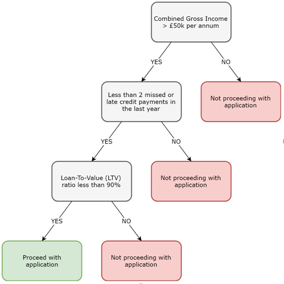
When traversing decision trees, start at the top. Thereafter, traverse left for yes, or positive responses, and traverse right for no, or negative responses. Once you reach the end of a branch, the leaf nodes describe the final outcome.

Case study – predicting political affiliation

For our next use case, we will use congressional voting records from the US House of Representatives to build a classification tree in order to predict whether a given congressman or woman is a Republican or a Democrat.

Note : 

The specific congressional voting dataset that we will use can be availed from UCI’s machine learning repository at https://archive.ics.uci.edu/ml/datasets/congressional+voting+records. It has been cited by Dua, D., and KarraTaniskidou, E. (2017). UCI Machine Learning Repository [http://archive.ics.uci.edu/ml]. Irvine, CA: University of California, School of Information and Computer Science.

If you open congressional-voting-data/house-votes-84.data in any text editor of your chice, you will find 435 congressional voting records, of which 267 belong to Democrats and 168 belong to Republicans. The first column contains the label string, in other words, Democrat or Republican, and the subsequent columns indicate how the congressman or woman in question voted on particular key issues at the time (y = for, n = against, ? = neither for nor against), such as an anti-satellite weapons test ban and a reduction in funding to a synthetic fuels corporation. Let’s now develop a classification tree in order to predict the political affiliation of a given congressman or woman based on their voting records:

Note :

The following sub-sections describe each of the pertinent cells in the corresponding Jupyter Notebook for this use case, entitled chp04-04-classification-regression-trees.ipynb, and which may be found at https://github.com/PacktPublishing/Machine-Learning-with-Apache-Spark-Quick-Start-Guide.  Note that for the sake of brevity, we will skip those cells that perform the same functions as seen previously.

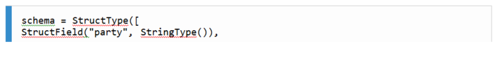
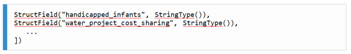
1. Since our raw data file has no header row, we need to explicitly define its schema before we can load it into a Spark DataFrame, as follows:

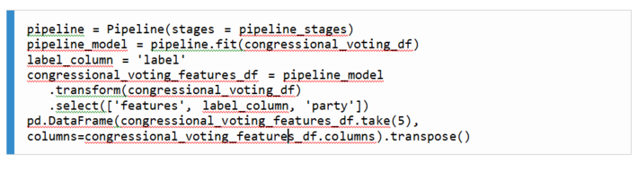
2. Since all of our columns, both the label and all the independent variables, are string-based data types, we need to apply a StringIndexer to them (as we did when developing our logistic regression model) in order to identify and index all possible categories for each column before generating numerical feature vectors. However, since we have multiple columns that we need to index, it is more efficient to build apipeline. A pipeline is a list of data and/or machine learning transformation stages to be applied to a Spark DataFrame. In our case, each stage in our pipeline will be the indexing of a different column as follows:

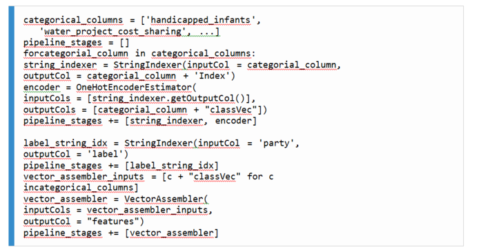
3. Next, we instantiate our pipeline by passing to it the list of stages that we generated in the previous cell. We then execute our pipeline on the raw Spark DataFrame using the fit() method, before proceeding to generate our numerical feature vectors using VectorAssembler as before:

4. We are now ready to train our classification tree! To achieve this, we can use MLlib’s DecisionTreeClassifier estimator to train a decision tree on our training dataset as follows:

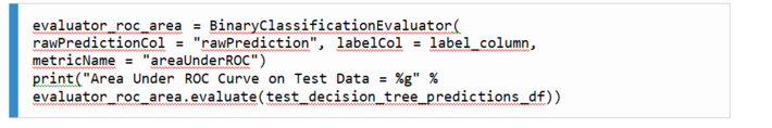
5. After training our classification tree, we will evaluate its performance on the test DataFrame. As with logistic regression, we can use the AUC metric as a measure of the proportion of time that the model predicts correctly. In our case, our model has an AUC metric of 0.91, which is very high:

6. Ideally, we would like to visualize our classification tree. Unfortunately, there is not yet any direct method in which to render a Spark decision tree without using third-party tools such as https://github.com/julioasotodv/spark-tree-plotting. However, we can render a text-based decision tree by invoking the toDebugString method on our trained classification tree model, as follows:

With an AUC value of 0.91, we can say that our classification tree model performs very well on the test data and is very good at predicting the political affiliation of congressmen and women based on their voting records. In fact, it classifies correctly 91% of the time across all threshold values!

Note that a CART model also generates probabilities, just like a logistic regression model. Therefore, we use a threshold value (default 0.5) in order to convert these probabilities into decisions, or classifications as in our example. There is, however, an added layer of complexity when it comes to training CART models—how do we control the number of splits in our decision tree?

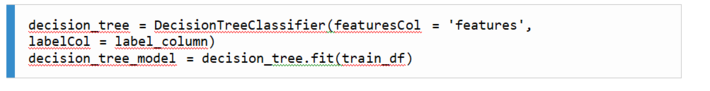
One method is to set a lower limit for the number of training data points to put into each subset or bucket. In MLlib, this value is tuneable, via the minInstancesPerNode parameter, which is accessible when training our DecisionTreeClassifier. The smaller this value, the more splits that will be generated.

However, if it is too small, then overfitting will occur. Conversely, if it is too large, then our CART model will be too simple with a low level of accuracy. We will discuss how to select an appropriate value during our introduction to random forests next. Note that MLlib also exposes other configurable parameters, including maxDepth (the maximum depth of the tree) and maxBins, but note that the larger a tree becomes in terms of splits and depth, the more computationally expensive it is to compute and traverse. To learn more about the tuneable parameters available to a DecisionTreeClassifier, please visit https://spark.apache.org/docs/latest/ml-classification-regression.html.

Random forests

One method of improving the accuracy of CART models is to build multiple decision trees, not just the one. In random forests, we do just that—a large number of CART trees are generated and thereafter, each tree in the forest votes on the outcome, with the majority outcome taken as the final prediction.

To generate a random forest, a process known as bootstrapping is employed whereby the training data for each tree making up the forest is selected randomly with replacement. Therefore, each individual tree will be trained using a different subset of independent variables and, hence, different training data.

K-Fold cross validation

Let’s now return to the challenge of choosing an appropriate lower-bound bucket size for an individual decision tree. This challenge is particularly pertinent when training a random forest since the computational complexity increases with the number of trees in the forest. To choose an appropriate minimum bucket size, we can employ a process known as K-Fold cross validation, the steps of which are as follows:

• Split a given training dataset into K subsets or “folds” of equal size.
• (K – 1) folds are then used to train the model, with the remaining fold, called the validation set, used to test the model and make predictions for each lower-bound bucket size value under consideration.
• This process is then repeated for all possible training and test fold combinations, resulting in the generation of multiple trained models that have been tested on each fold for every lower-bound bucket size value under consideration.
• For each lower-bound bucket size value under consideration, and for each fold, calculate the accuracy of the model on that combination pair.
• Finally, for each fold, plot the calculated accuracy of the model against each lower-bound bucket size value, as illustrated in Figure 4.8:

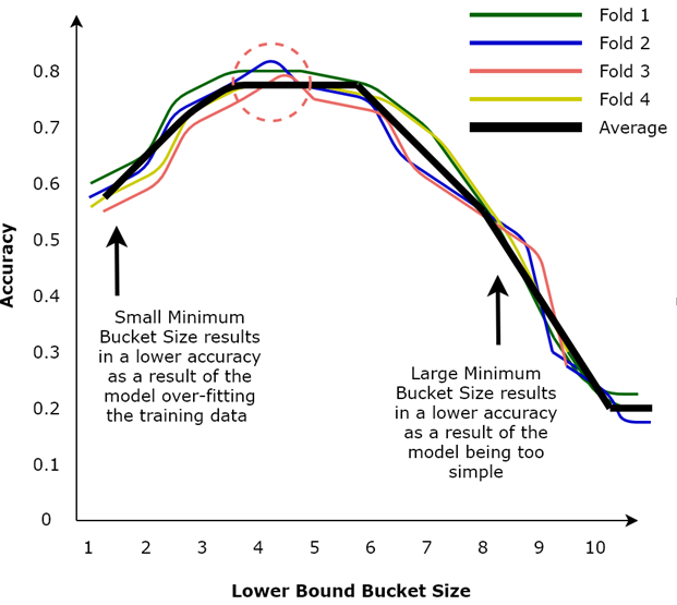
As illustrated in the above graph, choosing a small lower-bound bucket size value results in lower accuracy as a result of the model overfitting the training data. Conversely, choosing a large lower-bound bucket size value also results in lower accuracy as the model is too simple. Therefore, in our case, we would choose a lower-bound bucket size value of around 4 or 5, since the average accuracy of the model seems to be maximized in that region (as illustrated by the dashed circle in the above diagram).

Returning to our Jupyter Notebook, chp04-04-classification-regression-trees.ipynb, let’s now train a random forest model using the same congressional voting dataset to see whether it results in a better performing model compared to our single classification tree that we developed previously:

1. To build a random forest, we can use MLlib’s RandomForestClassifier estimator to train a random forest on our training dataset, specifying the minimum number of instances each child must have after a split via the minInstancesPerNode parameter, as follows:

2. We can now evaluate the performance of our trained random forest model on our test dataset by computing the AUC metric using the same BinaryClassificationEvaluator as follows:

Our trained random forest model has an AUC value of 0.97, meaning that it is more accurate in predicting political affiliation based on historical voting records than our single classification tree!

If you found this article helpful and would like to learn more about machine learning, you must explore Machine Learning with Apache Spark Quick Start Guide. Written by Jillur Quddus, Machine Learning with Apache Spark Quick Start Guide combines the latest scalable technologies with advanced analytical algorithms using real-world use-cases in order to derive actionable insights from Big Data in real-time.

Article originally posted on InfoQ. Visit InfoQ

Part of the async streams proposal is the ability to asynchronously dispose a resource. This interface is called IAsyncDisposable and has a single method called DisposeAsync. The first thing you may notice is the naming convention. Historically, the guidance from Microsoft is that asynchronous methods should end with the suffix “Async”. By contrast, the recommendation for types (i.e. classes and interfaces) is to use “Async” as a prefix.

As a potential performance improvement, DisposeAsync will return a ValueTask instead of a normal Task object. And because it may lead to instability, you will not be able to pass a cancellation token to the DisposeAsync method.

IDisposable vs IAsyncDisposable

IAsyncDisposable does not inherit from IDisposable, allowing developers to choose between implementing one or both interfaces. That said, the current theory is it is rare for a class to offer both interfaces.

Microsoft recommends that if you do have both, the class should allow Dispose and DisposeAsync to be called in either order. Only the first call will be honored, with subsequent calls to either method being a no-op. (This is only a recommendation; specific implementations may differ.)

Asynchronously Disposable Classes

Several classes have been singled out as needing asynchronous disposal support in .NET Core 3.0.

The first is Stream. This base class is used for a variety of scenarios and is often subclassed in third party libraries. The default implementation of AsyncDispose will be to call Dispose on a separate thread. This is generally considered to be a bad practice, so subclasses should override this behavior with a more appropriate implementation.

Likewise, a BinaryReader or TextReader will call Dispose on a separate thread if not overridden.

Threading.Timer has already implemented IAsyncDisposable as part of .NET Core 3.0.

CancellationTokenRegistration:

CancellationTokenRegistration.Dispose does two things: it unregisters the callback, and then it blocks until the callback has completed if the callback is currently running. DisposeAsync will do the same thing, but allow for that waiting to be done asynchronously rather than synchronously.

Changes to IAsyncEnumerator

Since we last reported on IAsyncEnumerator, the MoveNextAsync method has also been changed to return a ValueTask<bool>. This should allow for better performance in tight loops where MoveNextAsync will return synchronously most of the time.

Alternate Design for IAsyncEnumerator

An alternate design for IAsyncEnumerator was considered. Rather than a Current property like IEumerator, it would expose a method with this signature:

T TryGetNext(out bool success);

The success parameter indicates whether or not a value could be read synchronously. If it is false, the result of the function should be discarded and MoveNextAsync called to wait for more data.

Normally a try method returns a Boolean and the actual value is in an out parameter. However, that makes the method non-covariant (i.e. you cannot use IAsyncEnumerator<out T>), so the non-standard ordering was necessary.

This design was placed on hold for two reasons. First, the performance benefits during testing were not compelling. Using this pattern does improve performance, but those improvements are likely to be very minor in real world usage. Furthermore, this pattern is much harder to correctly use from both the library author’s and the client’s perspectives.

If the performance benefit is determined to be significant at a later date, then an optional second interface can be added to support that scenario.

Cancellation Tokens and Async Enumeration

It was decided that the IAsyncEnumerable<T>/IAsyncEnumerator<T> would be cancellation-agnostic. This means they cannot accept a cancellation token, nor would the new async aware for-each syntax have a way to directly consume one.

This doesn’t mean you cannot use cancellation tokens, only that there isn’t any special syntax to help you. You can still explicitly call ThrowIfCancellationRequested or pass a cancellation token to an iterator.

For-each Loops

For-each loops will continue to use the synchronous interfaces. In order to use the async enumerator, you must use the syntax below:

await foreach (var i in enumerable)

Note the placement of the await keyword. If you were to move it as shown in the next example, then getting the collection would be asynchronous, but the for-each loop itself would be synchronous.

foreach (var i in await enumerable)

Like a normal for-each loop, you do not need to actually implement the enumerator interfaces. If you expose instance (or extension) methods that match the async for-each pattern, they will be used even if the interfaces were also offered.

Article originally posted on InfoQ. Visit InfoQ

At the 2018 DevOps Summit in Las Vegas, Tapabrata “Topo” Pal, senior distinguished engineer, and Jamie Specter, counsel, presented how Capital One invested in open source in order to deploy software faster, and how they developed best practices based on their open source adoption’s lessons learned.

In 2012, Capital One was 100% Waterfall, had manual processes and out-sourced the majority of their commercial technology. In 6 years, Capital One became one of the largest digital banks, with millions of accounts, scaled DevOps across the organization, and in 2016 was named #1 company by Information Week Elite 100, a list that recognizes the best companies in technology innovation that drive real business value.

When they started their transformation journey, Capital One was opposed to open source. In 2012, they started developing their continuous integration pipeline with Apache Subversion, Jenkins, SonarQube, etc. But because of the risks posed by open source, they quickly engaged their legal department and together developed a formal due diligence approach and strategy. First, they identified and categorized all perceived risks associated with using open source software, such as security, trade secret disclosure, devaluation of patent portfolio, M&A devaluation, intellectual property infringement, etc. The key development risks were touching on security, licensing and reputation. They then identified a monitoring and remediation plan for each risk category, trained and empowered every employee involved in the process to act.

To prevent the code vulnerability and security risks, they developed a continuous detection model that decreased the remediation cycle time and quality. The remediation plan had 3 options, remove, replace or upgrade the code base. On the license front, there were over 2000 known open source licenses. Some licenses conflicted with each other, and some software had unknown licenses. It was important to understand the legal implications, permissions and rules as well as developers’ rights. Capital One established a continuous monitoring plan, enabling engineers to remove, rewrite or request a change of software quickly enough to have the least disruption possible. Capital One maintained an open source inventory, they continuously audited, tracked and remediated any vulnerabilities, tracked all license terms and established governance around technology, legal, security and training.

They also leveraged DevOps to help, through automation, small batch size, lean processes, frequent releases and high transparency. In 4 years, Capital One saw more than 90 developers working on 193 different projects using open source software such as Angular, Ansible and Kubernetes to simplify their automation, Hadoop, Kafka, etc. According to Pal and Specter, “you cannot do it alone”. They were successful because they removed silos in the enterprise, allowing engineers to collaborate faster with legal, security, and enterprise risks.

Capital One open source adoption took another turn, when, very soon into their transformation, in 2013, Pal realized and suggested that taping into existing open source only wasn’t going to provide them with all the benefits and innovation potential it offers. They went from being consumers to contributors. In 3 years, they developed their own open source portal, created 31 open source projects and products, among which Hygieia a DevOps dashboard, and Cloud Custodian are used today by many corporations.

According to Pal and Specter, creating a culture of open source was instrumental in meeting their organizational business and strategic goals. They improved their engineering skills and experience and saw an increase in software and release quality as well as in value to market.

Article originally posted on InfoQ. Visit InfoQ

XebiaLabs, a provider of DevOps and continuous delivery software tools, has launched new capabilities for custody, security and compliance risk assessment tracking for software releases via their DevOps Platform.

The new capabilities are intended to assist organisations to track application release status information and understand security and compliance risks across multiple different applications, teams, and environments. XebiaLabs say that when risk assessment, security testing, and compliance checks are not built into the continuous integration/continuous delivery (CI/CD) pipeline, releases can fail and cause delays, security vulnerabilities can threaten production, and IT governance violations can result in expensive fines. Derek Langone, CEO of XebiaLabs said:

To effectively manage software delivery at enterprise scale, DevOps teams need a way to accurately manage and report on the chain of custody and other compliance requirements throughout the software delivery pipeline. It’s also vital for them to have visibility into the risk of release failures or security issues as early in the release process as possible. That’s when development teams can address issues the quickest without impacting the business.

The XebiaLabs DevOps Platform provides visibility of the release chain of custody across the end-to-end CI/CD toolchain, from code to production. Teams can review security and compliance issues and take action to resolve release failure risks, security vulnerabilities, and IT governance violations are early in the software delivery cycle. XebiaLab’s chief product officer, Rob Stroud, provides a ‘chain of custody’ definition:

Chain of custody in software development refers to knowing the status of a release at any given moment: what’s in the release, what the components are, how they’re configured, who configured them, what gates have been successfully navigated, and which requirement the code derives from. You need to know the chain of custody of every release, so that if you’re ever in a situation where you must recreate or provide evidence in a discovery situation, you can be 100% certain that the information is correct. The information must be immutable and must provide the level of detail required to satisfy audit and regulatory requirements.

One of the features in the new release of XebiaLab’s DevOps Platform is enhanced chain of custody reporting that offers a deployment dashboard that shows what is being deployed, who is deploying it, and what the deployment status without dependency on which deployment tools are being used or what type of environments are being targeted. The environments can be on premise or private, public, or hybrid cloud. Users can see what is deployed where and track deployments back to feature development and delivery and can drill down into the chain of custody for completed releases to try to identify slow processes, bottlenecks, pain points, and areas for improvement and increased automation. The chain of custody shows which version of each application is deployed to each environment and tracks it back to which features are part of each application version.

The new release also includes a security risk dashboard for software releases that combines automated risk assessment for software delivery pipelines with security and compliance information from commonly used tools such as Black Duck, Fortify, SonarQube, and Checkmarx. Visualising security risk helps teams shift security and compliance activity left, so they can detect application vulnerabilities earlier and address them during development, before those vulnerabilities make it to production. Automatic trend analysis supports this capability further.

Also available are new ‘at-a-glance’ compliance overviews that summarise IT governance violations for common standards such as OWASP, PCI 3.2, and CWE/SANS and present compliance scanning activity and rule violations. Verifying security and compliance checks run for each release potentially accelerates audits and eases the load. The XebiaLabs Deployment dashboard and Security and Compliance dashboard are available now.

Article originally posted on Data Science Central. Visit Data Science Central

image source – wikipedia

We (Ajit Jaokar and Dan Howarth) are launching a new free online interactive book called Learn Machine Learning Coding Basics in a weekend

The idea is: spend one weekend to pick up the basics of coding for machine learning

The audience

1. Curious and already exploring machine learning online
2. Already can code in any language

The methodology

We are going to use deliberate practise to learn coding

I believe that this concept originated in the old soviet union athletes

It is also associated with a diverse range of people including Golf (Ben Hogan), Shaolin Monks, Benjamin Franklin etc. For the purposes of learning coding for machine learning, we apply the following elements of deliberate practice  

• Break down key ideas in simple, small steps. In this case, using a mindmap and a glossary
• Work with micro steps
• Keep the big picture in mind
• Encourage reflection/feedback
• Practice each element
• Reflect and adapt in microdata points
• Go slow

Image source: wikipedia

Artefacts / tools

• Mindmap – Glossary
• Colab
• Site of book posted for comments

This means we don’t need any installation (it’s completely web-based)

The process

Overview

We will guide you through two end-to-end machine learning problems that can be taken over one weekend. 

We will introduce you to important machine learning concepts, such as machine learning workflow, defining the problem statement, pre-processing and understanding our data, building baseline and more sophisticated models, and evaluating models. 

We will also introduce to keep machine learning libraries in python and demonstrate code that can be used on your own problems. We will cover data exploration in pandas, look at how to evaluate performance in numpy, plot our findings in Matplotlib, and build our models in sci-kit learn. 

Day 1 will focus on a regression problem and introduce you to the machine learning workflow and key libraries. We will build and evaluate our first models in sci-kit learn, and replicate our evaluation in numpy as a way of introducing you to the library. 

Day 2 will focus on a classification problem, and look to reinforce machine learning workflows, focus on pandas for data exploration and analysis, and build more models in sci-kit learn. We will end by building a machine learning pipeline. 
By the end of the weekend, you will have been introduced to core concepts and have some solid code examples that you can translate to new problems. We’ll also provide you with links to enable you to develop your knowledge further. 

Feedback mechanism

• comments in the comments section of the book
• we will aim to respond to in a week or the community can respond where possible.
• We are specifically interested in Missing concepts and Coding issues
• In keeping with the ideas of deliberate practise, we will narrow the focus and we will confine to the ideas in the notebooks

When

first week of Feb 2019

Interested?

Comment below and we will post link to book and code when live

Article originally posted on InfoQ. Visit InfoQ

If you look through the list of issues tagged for System.Collections in .NET 3.0, you’ll find both proposals that were accepted and rejected. In this report we’ll cover some of the highlights.

IList<T>.RemoveAll and Default Interface Methods

While IList<T> has a way to remove items by identity or index, it doesn’t provide an efficient way of removing items according to a predicate. Theoretically this missing method could be added in new versions of .NET without introducing a breaking change. This can be done through the use of a default interface method.

The first step towards this is support for default interface methods in .NET Standard 2.1. This feature, however, will not be offered for .NET Framework 4.8, which is thought to be the last major version of the original .NET Framework.

As a result, if IList<T> were modified then .NET Standard and .NET Framework would have different versions forever. In turn this means anything that implements IList<T> explicitly would have to differentiated using #if blocks. An implicit implementation of the interface, or just allowing for the default implementation, should be ok in this scenario.

For now, there are no immediate plans to actually use default interface methods even if they are offered in .NET Standard 2.1. Other issues, such as support in languages other than C#, still need to be considered. Immo Landwerth, a program manager at Microsoft, says, “when VB and F# offer full support for them, we’ll leverage them in the BCL.”

Optimizing BitArray

SSE2, also known as Streaming SIMD Extensions 2, is an old CPU technology dating back to the year 2000. Though it can offer significant performance when working with large sets of data, adoption has been slow. For example, SSE2 support wasn’t enabled by default in Visual C++ until 2012. And in the .NET world, Mono gained support for SIMD code in 2008, long before Microsoft’s .NET implementation offered it.

For a BitArray, using SSE2 can see a significant performance boost for large arrays. When testing a binary OR operation over 1000 integers, the average time dropped from 654.6 ns to 169.8 ns. These gains are far less impressive for small arrays and using SSE2 can be slower when working with less than 8 integers (256 bits). You can see the special handling used for small arrays as well as the SSE2 code itself in the pull request.

Span<T> is also being used to optimize BitArray. Unlike SSE2, the changes needed to use Span<T> often simplify the code as well.

Immutable Collection Builders and the Pit of Success

A core concept in .NET API design is what’s known as the “pit of success”. The basic concept is that an API should make it inconvenient or even hard to use a class incorrectly. Conversely, the easiest thing to do is most often the correct thing to do. You can see an example of this in proposal #21055.

When working with immutable collections, it is often advantageous to start by populating a mutable “builder” object. When you are done with your ImmutableArray.Builder, ImmutableDictionary.Builder, etc. then you are supposed to call ToImmutable() to freeze it into the corresponding immutable collection type.

However, if you are using any other kind of collection as a source then you need to call IEnumerable<T>.ToImmutableArray(), IEnumerable<T>.ToImmutableDictionary(), etc. These are generic extension methods and thus are slower than using the builder’s native ToImmutable() method. But from habit and consistency, most developers use the extension method and may not even know there is a better option.

In order to create a pit of success, ImmutableArray.Builder and friends are adding corresponding ToImmutableXxx methods that simply redirect the call to the correct ToImmutable() method. Since they are being added as instance methods, each supersedes the extension method with the same name.

Removing Items While Enumerating a Dictionary

Removing items from a collection is often frustrating because collections cannot normally be modified while they are being enumerated. If you modify the collection in any way, the enumerator is marked as invalid and must be discarded.

The work around is to create a copy of the collection. This copy is enumerated, allowing the original to be changed. However, this can be expensive, especially in the case of a Dictionary<K,V> where hash codes would need be calculated twice.

The aforementioned enumerator invalidation is handled by an internal field called “version”. Simply by not incrementing the version number when an item is removed, the need to make a preemptive copy is eliminated.

Meanwhile, a version increment was added to the TrimExcess() and EnsureCapacity() methods, as these “could modify the backing storage in such a way that they could break enumeration.” This may result in a breaking change if either method is called inside a for-each loop.

ObservableCollection, AddRange, and WPF

A common complaint about the Collection<T> and ObservableCollection<T> classes is the lack of an AddRange method. Found on the List<T> class, this method would allow for a much more efficient combining of collections than you would see when adding one item at a time in a loop. Other methods in the group include InsertRange, RemoveRange, and ReplaceRange.

At first glance it seems like it would be simple enough to add the missing methods. In the case of ObservableCollection<T>, the CollectionChanged event already allows you to indicate multiple items were added or removed at one time.

The problem with the “easy fix” is WPF. Due to a design flaw dating back over a decade, most of the built-in controls dealing with collections are incapable of processing collection changed events that refer to more than one item at a time. Rather than programming to the interface, WPF was designed only to work with the specific implementation of ObservableCollection<T>. Which means changes to it such as adding the AddRange method is akin to a breaking change.

The request to fix WPF so that it correctly handles collection changed events is tagged as a future enhancement. Meanwhile the design details for adding range methods to Collection<T> and ObservableCollection<T> continue to be debated.

Article originally posted on Data Science Central. Visit Data Science Central

This article is about Intuitive explanation of Degrees of Freedom and How Degrees of Freedom affects Sudoku.

A lot of aspiring Data Scientists take courses on statistics and get befuddled with the concept of Degrees of Freedom. Some memorize it by rote as ‘n-1′.

But there is a intuitive reason why it is ‘n-1’.

The Intuitive Explanation

Let’s consider the following example.

Imagine being asked to choose 5 numbers that sum to 100. For simplicity sake, you say 20, 20, 20, 20. Before you utter the 5th number, I tell you that your 5th number is 20 as well. This is because the first 4 numbers chosen by you summed up to 80 and the condition was to chose 5 numbers which sum to 100.

So 100 -80 = 20. The fifth number is 20.

The fifth number in a sense chose itself due to the condition specified.

You see you had 4 degrees of freedom alone. All one needed was the first four numbers.

This also intuitively explains the n-1. Here n being 5 and n-1 =4.

You lost one degree of freedom to the condition of “5 numbers should sum to 100”

or

In other words, you had 4 degrees of freedom.

The Sudoku Connection

Sudoku is a very familiar game to most of us. Wikipedia gives the following definition

Sudoku originally called Number Place)is a logic-based, combinatorial number-placement puzzle. The objective is to fill a 9×9 grid with digits so that each column, each row, and each of the nine 3×3 subgrids that compose the grid (also called “boxes”, “blocks”, or “regions”) contains all of the digits from 1 to 9. The puzzle setter provides a partially completed grid, which for a well-posed puzzle has a single solution.

I was solving a sudoku game just to kill some time. I realized that there is some connection between sudoku and degrees of freedom.

I am not sure whether the online version of the game takes into account degrees of freedom to rate the game as “Easy”, “Medium” and“Expert”. But perhaps the game could be rated this way !!

Let me illustrate with an example taken from an online sudoku puzzle.

The ‘Easy’, ‘Medium’, ‘Hard’ and “Evil’ levels of online sudoku game is depicted below.

Note there are 81 cells in a Sudoku game.