In the beginning, learning Machine Learning (ML) can be intimidating. Terms like “Gradient Descent”, “Latent Dirichlet Allocation” or “Convolutional Layer” can scare lots of people. But there are friendly ways of getting into the discipline, and I think starting with Decision Trees is a wise decision.

Decision Trees (DTs) are probably one of the most useful supervised learningalgorithms out there. As opposed to unsupervised learning (where there is no output variable to guide the learning process and data is explored by algorithms to find patterns), in supervised learning your existing data is already labelled and you know which behaviour you want to predict in the new data you obtain. This is the type of algorithms that autonomous cars use to recognize pedestrians and objects, or organizations exploit to estimate customers lifetime value and their churn rates.

In a way, supervised learning is like learning with a teacher, and then apply that knowledge to new data.

DTs are ML algorithms that progressively divide data sets into smaller data groups based on a descriptive feature, until they reach sets that are small enough to be described by some label. They require that you have data that is labelled (tagged with one or more labels, like the plant name in pictures of plants), so they try to label new data based on that knowledge.

DTs algorithms are perfect to solve classification (where machines sort data into classes, like whether an email is spam or not) and regression (where machines predict values, like a property price) problems. Regression Trees are used when the dependent variable is continuous or quantitative (e.g. if we want to estimate the probability that a customer will default on a loan), and Classification Trees are used when the dependent variable is categorical or qualitative (e.g. if we want to estimate the blood type of a person).

The importance of DTs relies on the fact that they have lots of applications in the real world. Being one of the mostly used algorithms in ML, they are applied to different functionalities in several industries:

• DTs are being used in the healthcare industry to improve the screening of positive cases in the early detection of cognitive impairment, and also to identify the main risk factors of developing some type of dementia in the future.
• Sophia, the robot that was made a citizen of Saudi Arabia, uses DTs algorithms to chat with humans. In fact, chatbots that use these algorithms are already bringing benefits in industries like health insuranceby gathering data from customers through the application of innovative surveys and friendly chats. Google recently acquired Onward, a company that uses DTs to develop chatbots that are exceptionally functional in delivering world-class customer care, and Amazon is investing in the same direction to guide customers quickly to a path of resolution.
• It is possible to predict the most likely causes of forest disturbances, like wildfire, logging of tree plantations, large or small scale agriculture, and urbanization by training DTs to recognize different causes of forest lossfrom satellite imagery. DTs and satellite imagery are also used in agriculture to classify different crop types and identify their phenological stages.
• DTs are great tools to perform sentiment analysis of texts, and identify the emotions behind them. Sentiment analysis is a powerful technique that can help organizations to learn about customers choices and their decision drivers.
• In environmental sciences, DTs can help to determine the best strategy for dealing with invasive species, ranging from eradication to containment, and mitigation of spread.
• DTs are also used to improve financial fraud detection. The MIT showed that it could significantly improve the performance of alternative ML models by using DTs that were trained with several sources of raw data to find patterns of transactions and credit cards that match cases of fraud.

DTs are extremely popular for a variety of reasons, being their interpretability probably their most important advantage. They can be trained very fast and are easy to understand, which opens their possibilities to frontiers far beyond scientific walls. Nowadays, DTs are very popular in business environments and their usage is also expanding to civil areas, where some applications are raising big concerns.

The firm Sesame Credit (a company affiliated with Alibaba) uses DTs and other algorithms to engine a system of social evaluation, taking into consideration various factors such as the punctuality with which bills are paid and other online activities. The benefits of a good “Sesame score” in China range from a higher visibility on dating sites to skipping the waiting line if you need to see a doctor. Actually, after the chinese government announced it will apply its so-called social credit system to flights and trains and stop people who have committed misdeeds from taking such transport for up to a year, there is a concern that the system will end up creating a massive “ML-backed Big Brother”.

The Basics

In the movie Bandersnatch (a stand-alone Black Mirror episode from Netflix), the viewer can interactively choose different narrative paths and reach different story lines and endings. There is a complex set of decisions hidden behind the movie storytelling that lets the audience move in a kind of Choose Your Own Adventure mode, for which Netflix had to work out a way of loading multiple versions of each scene while presenting it in a simple way. In practice, what Netflix producers did was to segment the movie and set different branch points for the viewer to move through, and come up with different results. In other words, this is just like building a DT.

DTs are composed of nodes, branches and leafs. Each node represents an attribute (or feature), each branch represents a rule (or decision), and eachleaf represents an outcome. The depth of a Tree is defined by the number of levels, not including the root node.

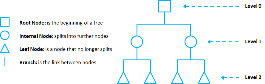
In this example, a DT of 2 levels.

DTs apply a top-down approach to data, so that given a data set, they try to group and label observations that are similar between them, and look for the best rules that split the observations that are dissimilar between them until they reach certain degree of similarity.

They use a layered splitting process, where at each layer they try to split the data into two or more groups, so that data that fall into the same group are most similar to each other (homogeneity), and groups are as different as possible from each other (heterogeneity).

The splitting can be binary (which splits each node into at most two sub-groups, and tries to find the optimal partitioning), or multiway (which splits each node into multiple sub-groups, using as many partitions as existing distinct values). In practice, it is usual to see DTs with binary splits, but it’s important to know that multiway splitting has some advantages. Multiway splits exhaust all information in a nominal attribute, which means that an attribute rarely appears more than once in any path from the root to the leaf, which make DTs easier to comprehend. In fact, it could happen that the best way to split data might be to find a set of intervals for a given feature, and then split that data up into several groups based on those intervals.

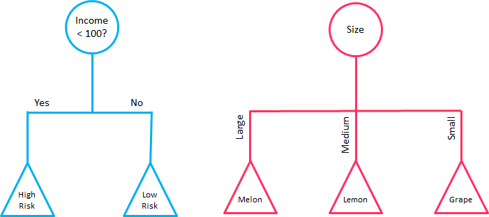
On the left hand side, a DT with binary splitting, as opposed to a DT with multiway splitting on the right.

In bidimensional terms (using only 2 variables), DTs partition the data universe into a set of rectangles, and fit a model in each one of those rectangles. They are simple yet powerful, and a great tool for data scientists.

Right figure shows the partition of the bidimensional data space produced by the DT on the left (binary split). In practice, however, DTs use numerous variables (usually more than 2).

Each node in the DT acts as a test case for some condition, and each branch descending from that node corresponds to one of the possible answers to that test case.

Prune that Tree

As the number of splits in DTs increase, their complexity rises. In general, simpler DTs are preferred over super complex ones, since they are easier to understand and they are less likely to fall into overfitting.

Overfitting refers to a model that learns the training data(the data it uses to learn) so well that it has problems to generalize to new (unseen) data.

In other words, the model learns the detail and noise (irrelevant information or randomness in a dataset) in the training data to the extent that it negatively impacts the performance of the model on new data. This means that the noise or random fluctuations in the training data is picked up and learned as concepts by the model.

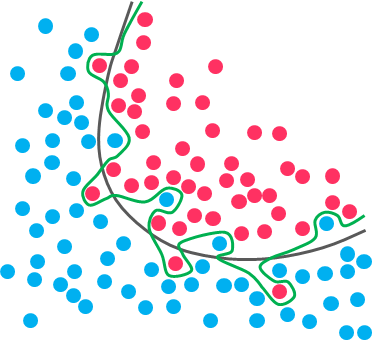
While the black line fits the data well, the green line is overfitting

Under this condition, your model works perfectly well with the data you provide upfront, but when you expose that same model to new data, it breaks down. It’s unable to repeat its highly detailed performance.

So, how do you avoid overfitting in DTs? You need to exclude branches that fit data too specifically. You want a DT that can generalize and work well on new data, even though this may imply losing precision on the training data. It’s always better to avoid a DT model that learns and repeats specific details like a parrot, and try to develop one that has the power and flexibility to have a decent performance on new data you provide to it.

Pruning is a technique used to deal with overfitting, that reduces the size of DTs by removing sections of the Tree that provide little predictive or classification power.

The goal of this procedure is to reduce complexity and gain better accuracy by reducing the effects of overfitting and removing sections of the DT that may be based on noisy or erroneous data. There are two different strategies to perform pruning on DTs:

• Pre-prune: When you stop growing DT branches when information becomes unreliable.
• Post-prune: When you take a fully grown DT and then remove leaf nodes only if it results in a better model performance. This way, you stop removing nodes when no further improvements can be made.

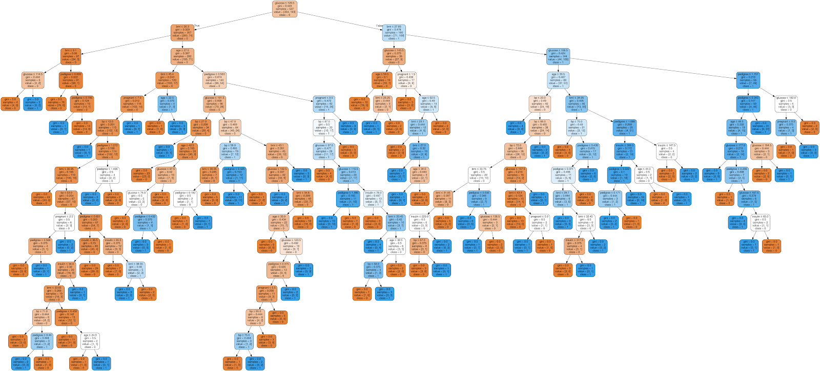
Example of an unpruned DT, as taken from DataCamp

In summary, a big DT that correctly classifies or predicts every example of the training data might not be as good as a smaller one that does not fit all the training data perfectly.

Main DTs algorithms

Now you may ask yourself: how do DTs know which features to select and how to split the data? To understand that, we need to get into some details.

All DTs perform basically the same task: they examine all the attributes of the dataset to find the ones that give the best possible result by splitting the data into subgroups. They perform this task recursively by splitting subgroups into smaller and smaller units until the Tree is finished (stopped by certain criteria).

This decision of making splits heavily affects the Tree’s accuracy and performance, and for that decision, DTs can use different algorithms that differ in the possible structure of the Tree (e.g. the number of splits per node), the criteria on how to perform the splits, and when to stop splitting.

So, how can we define which attributes to split, when and how to split them? To answer this question, we must review the main DTs algorithms:

CHAID

The Chi-squared Automatic Interaction Detection (CHAID) is one of the oldest DT algorithms methods that produces multiway DTs (splits can have more than two branches) suitable for classification and regression tasks. When building Classification Trees (where the dependent variable is categorical in nature), CHAID relies on the Chi-square independence tests to determine the best split at each step. Chi-square tests check if there is a relationship between two variables, and are applied at each stage of the DT to ensure that each branch is significantly associated with a statistically significant predictor of the response variable.

In other words, it chooses the independent variable that has the strongest interaction with the dependent variable.

Additionally, categories of each predictor are merged if they are not significantly different between each other, with respect to the dependent variable. In the case of Regression Trees (where the dependent variable is continuous), CHAID relies on F-tests (instead of Chi-square tests) to calculate the difference between two population means. If the F-test is significant, a new partition (child node) is created (which means that the partition is statistically different from the parent node). On the other hand, if the result of the F-test between target means is not significant, the categories are merged into a single node.

CHAID does not replace missing values and handles them as a single class which may merge with another class if appropriate. It also produces DTs that tend to be wider rather than deeper (multiway characteristic), which may be unrealistically short and hard to relate to real business conditions. Additionally, it has no pruning function.

Although not the most powerful (in terms of detecting the smallest possible differences) or fastest DT algorithm out there, CHAID is easy to manage, flexible and can be very useful.

You can find an implementation of CHAID with R in this link

CART

CART is a DT algorithm that produces binary Classification or RegressionTrees, depending on whether the dependent (or target) variable is categorical or numeric, respectively. It handles data in its raw form (no preprocessing needed), and can use the same variables more than once in different parts of the same DT, which may uncover complex interdependencies between sets of variables.

In the case of Classification Trees, CART algorithm uses a metric called Gini Impurity to create decision points for classification tasks. Gini Impurity gives an idea of how fine a split is (a measure of a node’s “purity”), by how mixed the classes are in the two groups created by the split. When all observations belong to the same label, there’s a perfect classification and a Gini Impurity value of 0 (minimum value). On the other hand, when all observations are equally distributed among different labels, we face the worst case split result and a Gini Impurity value of 1 (maximum value).

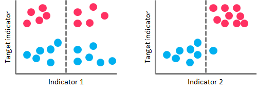
On the left-hand side, a high Gini Impurity value leads to a poor splitting performance. On the right-hand side, a low Gini Impurity value performs a nearly perfect splitting

In the case of Regression Trees, CART algorithm looks for splits that minimize the Least Square Deviation (LSD), choosing the partitions that minimize the result over all possible options. The LSD (sometimes referred as “variance reduction”) metric minimizes the sum of the squared distances (or deviations) between the observed values and the predicted values. The difference between the predicted and observed values is called “residual”, which means that LSD chooses the parameter estimates so that the sum of the squared residuals is minimized.

LSD is well suited for metric data and has the ability to correctly capture more information about the quality of the split than other algorithms.

The idea behind CART algorithm is to produce a sequence of DTs, each of which is a candidate to be the “optimal Tree”. This optimal Tree is identified by evaluating the performance of every Tree through testing (using new data, which the DT has never seen before) or performing cross-validation(dividing the dataset into “k” number of folds, and perform testings on each fold).

CART doesn’t use an internal performance measure for Tree selection. Instead, DTs performances are always measured through testing or via cross-validation, and the Tree selection proceeds only after this evaluation has been done.

ID3

The Iterative Dichotomiser 3 (ID3) is a DT algorithm that is mainly used to produce Classification Trees. Since it hasn’t proved to be so effective building Regression Trees in its raw data, ID3 is mostly used for classification tasks (although some techniques such as building numerical intervals can improve its performance on Regression Trees).

ID3 splits data attributes (dichotomizes) to find the most dominant features, performing this process iteratively to select the DT nodes in a top-down approach.

For the splitting process, ID3 uses the Information Gain metric to select the most useful attributes for classification. Information Gain is a concept extracted from Information Theory, that refers to the decrease in the level of randomness in a set of data: basically it measures how much “information” a feature gives us about a class. ID3 will always try to maximize this metric, which means that the attribute with the highest Information Gain will split first.

Information Gain is directly linked to the concept of Entropy, which is the measure of the amount of uncertainty or randomness in the data. Entropy values range from 0 (when all members belong to the same class or the sample is completely homogeneous) to 1 (when there is perfect randomness or unpredictability, or the sample is equally divided).

You can think it this way: if you want to make an unbiased coin toss, there is complete randomness or an Entropy value of 1 (“heads” and “tails” are equally like, with a probability of 0.5 each). On the other hand, if you make a coin toss, with for example a coin that has “tails” on both sides, randomness is removed from the event and the Entropy value is 0 (probability of getting “tails” will jump to 1, and probability of “heads” will drop to 0).

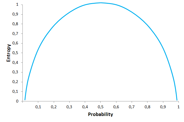
In this graph you can see the relationship between Entropy and the probability of different coin tosses. At the highest level of Entropy, the probability of getting “tails” is equal to the one of getting “heads” (0.5 each), and we face complete uncertainty. Entropy is directly linked to the probability of an event. Example taken from The Null Pointer Exception

This is important because Information Gain is the decrease in Entropy, and the attribute that yields the largest Information Gain is chosen for the DT node.

But ID3 has some disadvantages: it can’t handle numeric attributes nor missing values, which can represent serious limitations.

C4.5

C4.5 is the successor of ID3 and represents an improvement in several aspects. C4.5 can handle both continuous and categorical data, making it suitable to generate Regression and Classification Trees. Additionally, it can deal with missing values by ignoring instances that include non-existing data.

Unlike ID3 (which uses Information Gain as splitting criteria), C4.5 uses Gain Ratio for its splitting process. Gain Ratio is a modification of the Information Gain concept that reduces the bias on DTs with huge amount of branches, by taking into account the number and size of the branches when choosing an attribute. Since Information Gain shows an unfair favoritism towards attributes with many outcomes, Gain Ratio corrects this trend by considering the intrinsic information of each split (it basically “normalizes” the Information Gain by using a split information value). This way, the attribute with the maximum Gain Ratio is selected as the splitting attribute.

Additionally, C4.5 includes a technique called windowing, which was originally developed to overcome the memory limitations of earlier computers. Windowing means that the algorithm randomly selects a subset of the training data (called a “window”) and builds a DT from that selection. This DT is then used to classify the remaining training data, and if it performs a correct classification, the DT is finished. Otherwise, all the misclassified data points are added to the windows, and the cycle repeats until every instance in the training set is correctly classified by the current DT. This technique generally results in DTs that are more accurate than those produced by the standard process due to the use of randomization, since it captures all the “rare” instances together with sufficient “ordinary” cases.

Another capability of C4.5 is that it can prune DTs.

C4.5’s pruning method is based on estimating the error rate of every internal node, and replacing it with a leaf node if the estimated error of the leaf is lower. In simple terms, if the algorithm estimates that the DT will be more accurate if the “children” of a node are deleted and that node is made a leaf node, then C4.5 will delete those children.

The latest version of this algorithm is called C5.0, which was released under proprietary license and presents some improvements over C4.5 like:

• Improved speed: C5.0 is significantly faster than C4.5 (by several orders of magnitude).
• Memory usage: C5.0 is more memory efficient than C4.5.
• Variable misclassification costs: in C4.5 all errors are treated as equal, but in practical applications some classification errors are more serious than others. C5.0 allows to define separate cost for each predicted/actual class pair.
• Smaller decision trees: C5.0 gets similar results to C4.5 with considerably smaller DTs.
• Additional data types: C5.0 can work with dates, times, and allows values to be noted as “not applicable”.
• Winnowing: C5.0 can automatically winnow the attributes before a classifier is constructed, discarding those that may be unhelpful or seem irrelevant.

You can find a comparison between C4.5 and C5.0 here

The dark side of the Tree

Surely DTs have lots of advantages. Because of their simplicity and the fact that they are easy to understand and implement, they are widely used for different solutions in a large number of industries. But you also need to be aware of its disadvantages.

DTs tend to overfit on their training data, making them perform badly if data previously shown to them doesn’t match to what they are shown later.

They also suffer from high variance, which means that a small change in the data can result in a very different set of splits, making interpretation somewhat complex. They suffer from an inherent instability, since due to their hierarchical nature, the effect of an error in the top splits propagate down to all of the splits below.

In Classification Trees, the consequences of misclassifying observations are more serious in some classes than others. For example, it is probably worse to predict that a person will not have a heart attack when he/she actually will, than vice versa. This problem is mitigated in algorithms like C5.0, but remains as a serious issue in others.

DTs can also create biased Trees if some classes dominate over others. This is a problem in unbalanced datasets (where different classes in the dataset have different number of observations), in which case it is recommended to balance de dataset prior to building the DT.

In the case of Regression Trees, DTs can only predict within the range of values they created based on the data they saw before, which means that they have boundaries on the values they can produce.

At each level, DTs look for the best possible split so that they optimize the corresponding splitting criteria.

But DTs splitting algorithms can’t see far beyond the current level in which they are operating (they are “greedy”), which means that they look for a locally optimal and not a globally optimal at each step.

DTs algorithms grow Trees one node at a time according to some splitting criteria and don’t implement any backtracking technique.

The power of the crowd

But here are the good news: there are different strategies to overcome these drawbacks. Ensemble methods combine several DTs to improve the performance of single DTs, and are a great resource to get over the problems already described. The idea is to train multiple models using the same learning algorithm to achieve superior results.

Probably the 2 most common techniques to perform ensemble DTs are Bagging and Boosting.

Bagging (or Bootstrap Aggregation) is used when the goal is to reduce the variance of a DT. Variance relates to the fact that DTs can be quite unstable because small variations in the data might result in a completely different Tree being generated. So, the idea of Bagging is to solve this issue by creating in parallel random subsets of data (from the training data), where any observation has the same probability to appear in a new subset data. Next, each collection of subset data is used to train DTs, resulting in an ensemble of different DTs. Finally, an average of all predictions of those different DTs is used, which produces a more robust performance than single DTs. Random Forest is an extension over Bagging, which takes one extra step: in addition to taking the random subset of data, it also takes a random selection of features rather than using all features to grow DTs.

Boosting is another technique that creates a collection of predictors to reduce the variance of a DT, but with a different approach. It uses a sequential method where it fits consecutive DTS, and at every step, tries to reduce the errors from the prior Tree. With Boosting techniques, each classifier is trained on data, taking into account the previous classifier success. After each training step, the weights are redistributed based on the previous performance. This way, misclassified data increases its weights to emphasize the most difficult cases, so that subsequent DTs will focus on them during their training stage and improve their accuracy. Unlike Bagging, in Boosting the observations are weighted and therefore some of them will take part in the new subsets of data more often. As a result of this process, the combination of the whole sets improves the performance of DTs.

Within Boosting, there are several alternatives to determine the weights to use in the training and classification steps (e.g. Gradient Boost, XGBoost, AdaBoost, and others).

You can find a description of similarities and differences between both techniques here

Interested in these topics? Follow me on Linkedin or Twitter

Let’s say you want to classify hundreds (or thousands) of documents based on their content and topics, or you wish to group together different images for some reason. Or what’s even more, let’s think you have that same data already classified but you want to challenge that labeling. You want to know if that data categorization makes sense or not, or can be improved.

Well, my advice is that you cluster your data. Information is often darkened by noise and redundancy, and grouping data into clusters (clustering) with similar features is an efficient way to bring some light on.

Clustering is a technique widely used to find groups of observations (called clusters) that share similar characteristics. This process is not driven by a specific purpose, which means you don’t have to specifically tell your algorithm how to group those observations since it does it on its own (groups are formed organically). The result is that observations (or data points) in the same group are more similar between them than other observations in another group. The goal is to obtain data points in the same group as similar as possible, and data points in different groups as dissimilar as possible.

Extremely well fitted for exploratory analysis, K-means is perfect for getting to know your data and providing insights on almost all datatypes. Whether it is an image, a figure or a piece of text, K-means is so flexible it can take almost everything.

One of the rockstars in unsupervised learning

Clustering (including K-means clustering) is an unsupervised learning technique used for data classification.

Unsupervised learning means there is no output variable to guide the learning process (no this or that, no right or wrong) and data is explored by algorithms to find patterns. We only observe the features but have no established measurements of the outcomes since we want to find them out.

As opposed to supervised learning where your existing data is already labeled and you know which behaviour you want to determine in the new data youobtain, unsupervised learning techniques don’t use labelled data and the algorithms are left to themselves to discover structures in the data.

Within the universe of clustering techniques, K-means is probably one of the mostly known and frequently used. K-means uses an iterative refinement method to produce its final clustering based on the number of clusters defined by the user (represented by the variable K) and the dataset. For example, if you set K equal to 3 then your dataset will be grouped in 3 clusters, if you set K equal to 4 you will group the data in 4 clusters, and so on.

K-means starts off with arbitrarily chosen data points as proposed means of the data groups, and iteratively recalculates new means in order to converge to a final clustering of the data points.

But how does the algorithm decide how to group the data if you are just providing a value (K)? When you define the value of K you are actually telling the algorithm how many means or centroids you want (if you set K=3 you create 3 means or centroids, which accounts for 3 clusters). A centroid is a data point that represents the center of the cluster (the mean), and it might not necessarily be a member of the dataset.

This is how the algorithm works:

1. K centroids are created randomly (based on the predefined value of K)
2. K-means allocates every data point in the dataset to the nearest centroid (minimizing Euclidean distances between them), meaning that a data point is considered to be in a particular cluster if it is closer to that cluster’s centroid than any other centroid
3. Then K-means recalculates the centroids by taking the mean of all data points assigned to that centroid’s cluster, hence reducing the total intra-cluster variance in relation to the previous step. The “means” in the K-means refers to averaging the data and finding the new centroid
4. The algorithm iterates between steps 2 and 3 until some criteria is met (e.g. the sum of distances between the data points and their corresponding centroid is minimized, a maximum number of iterations is reached, no changes in centroids value or no data points change clusters)

In this example, after 5 iterations the calculated centroids remain the same, and data points are not switching clusters anymore (the algorithm converges). Here, each centroid is shown as a dark coloured data point. Source: http://ai.stanford.edu

The initial result of running this algorithm may not be the best possible outcome and rerunning it with different randomized starting centroids might provide a better performance (different initial objects may produce different clustering results). For this reason, it’s a common practice to run the algorithm multiple times with different starting points and evaluate different initiation methods (e.g. Forgy or Kaufman approaches).

But another question arises: how do you know the correct value of K, or how many centroids to create? There is no universal answer for this, and although the optimal number of centroids or clusters is not known a priori, different approaches exist to try to estimate it. One commonly used approach is testing different numbers of clusters and measure the resulting sum of squared errors, choosing the K value at which an increase will cause a very small decrease in the error sum, while a decrease will sharply increase the error sum. This point that defines the optimal number of clusters is known as the “elbow point”, and can be used as a visual measure to find the best pick for the value of K.

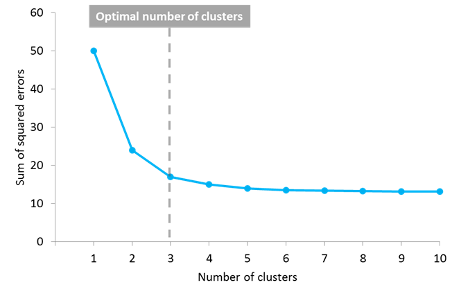
In this example, the elbow point is located in 3 clusters

K-means is a must-have in your data science toolkit, and there are several reasons for this. First of all it’s easy to implement and brings an efficient performance. After all, you need to define just one parameter (the value of K) to see the results. It is also fast and works really well with large datasets, making it capable of dealing with the current huge volumes of data. It’s soflexible that it can be used with pretty much any datatype and its results are easy to interpret and more explainable than other algorithms. Furthermore, the algorithm is so popular that you may find use cases and implementations in almost any discipline.

But everything has a downside

Nevertheless, K-means presents some disadvantages. The first one is that you need to define the number of clusters, and this decision can seriously affect the results. Also, as the location of the initial centroids is random, results may not be comparable and show lack of consistency. K-means produces clusters with uniform sizes (each cluster with roughly an equal quantity of observations), even though the data might behave in a different way, and it’s very sensitive to outliers and noisy data. Additionally, it assumes that data points in each cluster are modeled as located within a sphere around that cluster centroid (spherical limitation), but when this condition (or any of the previous ones) is violated, the algorithm can behave in non-intuitive ways.

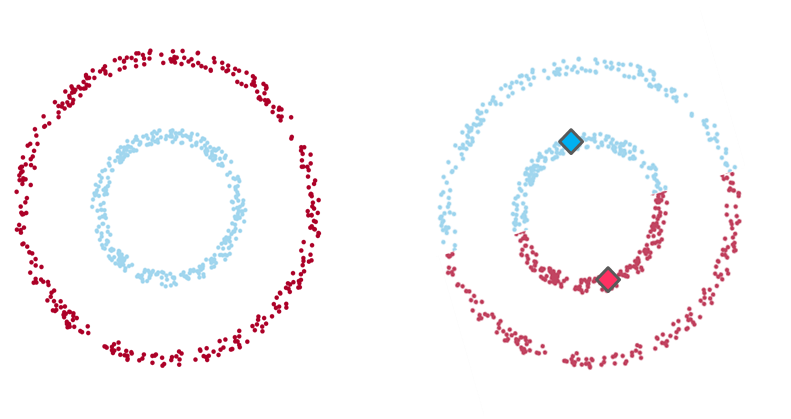
Example 1

Example 1: On the left-hand side the intuitive clustering of the data, with a clear separation between two groups of data points (in the shape of one small ring surrounded by a larger one). On the right-hand side, the same data points clustered by K-means algorithm (with a K value of 2), where each centroid is represented with a diamond shape. As you see, the algorithm fails to identify the intuitive clustering.

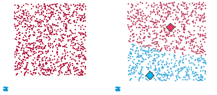
Example 2

Example 2: On the left-hand side the clustering of two recognizable data groups. On the right-hand side, the result of K-means clustering over the same data points does not fit the intuitive clustering. As in the case of example 1, K-means created partitions that don’t reflect what we visually identify due to the algorithm’s spherical limitation. It tries to find centroids with neat spheres of data around them, and performs badly as the cluster’s geometric shape deviates from a sphere.

Example 3

Example 3: Once again, on the left-hand side there are two clear clusters (one small and tight data group and another larger and dispersed one) which K-means fails to identify (right-hand side). Here, in an attempt to balance the intra-cluster distances between both data groups and generate clusters with uniform sizes, the algorithm blends both data groups and creates 2 artificial clusters that don’t represent the dataset.

It’s interesting to see that K-means doesn’t allow data points that are far away from each other to share the same cluster, no matter how obvious the relation between these data points might be.

What to do now?

The thing is real life data is almost always complex, disorganized and noisy. Situations in the real world rarely reflect clear conditions in which to apply these type of algorithms right out of the shelf. In the case of K-means algorithm it will be expected that at least one of its assumptions gets violated, so we need not only to identify this, but to know what to do in such case.

The good news is that there are alternatives, and deficiencies can be corrected. For example, converting data to polar coordinates can solve the spherical limitation we described in example 1. You may also consider using other types of clustering algorithms if you find serious limitations. Possible approaches would be to use density-based or hierarchical-based algorithms, which fix some of K-means limitations (but have their own limitations).

In summary, K-means is a wonderful algorithm with lots of potential uses, so versatile it can be used for almost any kind of data grouping. But there is never a free lunch: you need to be aware of its assumptions and the way it operates if you don’t want to get guided to wrong results.

Interested in these topics? Follow me on Linkedin or Twitter

R studio

Data structures

You’ve probably used many (if not all) of them before, but you may not have thought deeply about how they are interrelated. In this brief overview, I’ll show you how they fit together as a whole. If you need more details, you can find them in R’s documentation.

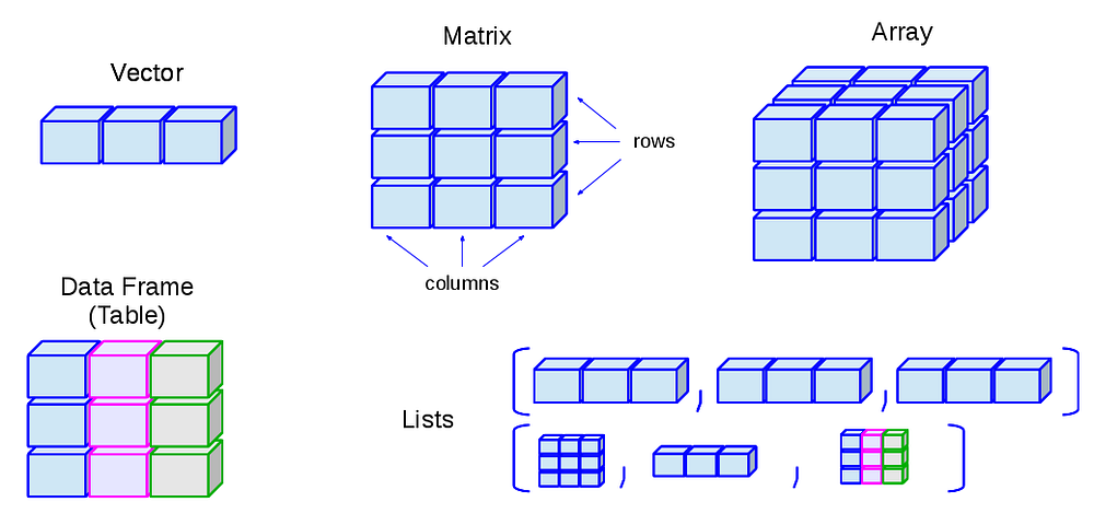
R’s base data structures can be organised by their dimensionality (1d, 2d, or nd) and whether they’re homogeneous (all contents must be of the same type) or heterogeneous (the contents can be of different types). This gives rise to the five data types most often used in data analysis:

Homogeneous: Atomic vector (1d), Matrix(2d), Array(nd)

Heterogeneous: List, Data frame

Hacker Noon

Almost all other objects are built upon these foundations. In the OO field guide you’ll see how more complicated objects are built of these simple pieces. Note that R has no 0-dimensional, or scalar types. Individual numbers or strings, which you might think would be scalars, are actually vectors of length one.

Given an object, the best way to understand what data structures it’s composed of is to use str(). str() is short for structure and it gives a compact, human readable description of any R data structure.

Almost all other objects are built upon these foundations. In the OO field guide you’ll see how more complicated objects are built of these simple pieces. Note that R has no 0-dimensional, or scalar types. Individual numbers or strings, which you might think would be scalars, are actually vectors of length one.

Given an object, the best way to understand what data structures it’s composed of is to use str(). str() is short for structure and it gives a compact, human readable description of any R data structure.

Vectors

The basic data structure in R is the vector. Vectors come in two flavours: atomic vectors and lists. They have three common properties:

• Type, typeof(), what it is.
• Length, length(), how many elements it contains.
• Attributes, attributes(), additional arbitrary metadata.

They differ in the types of their elements: all elements of an atomic vector must be the same type, whereas the elements of a list can have different types.

NB: is.vector() does not test if an object is a vector. Instead it returns TRUEonly if the object is a vector with no attributes apart from names. Use is.atomic(x) || is.list(x) to test if an object is actually a vector.

Atomic vectors

There are four common types of atomic vectors that I’ll discuss in detail: logical, integer, double (often called numeric), and character. There are two rare types that I will not discuss further: complex and raw.

Atomic vectors are usually created with c(), short for combine:

dbl_var <- c(1, 2.5, 4.5)
# With the L suffix, you get an integer rather than a double

int_var <- c(1L, 6L, 10L)
# Use TRUE and FALSE (or T and F) to create logical vectors

log_var <- c(TRUE, FALSE, T, F)

chr_var <- c("these are", "some strings")

Atomic vectors are always flat, even if you nest c()’s:

c(1, c(2, c(3, 4)))

## [1] 1 2 3 4

# the same as
c(1, 2, 3, 4)

## [1] 1 2 3 4

Missing values are specified with NA, which is a logical vector of length 1. NAwill always be coerced to the correct type if used inside c(), or you can create NAs of a specific type with NA_real_ (a double vector), NA_integer_ and NA_character_.

Types and tests

Given a vector, you can determine its type with typeof(), or check if it’s a specific type with an “is” function: is.character(), is.double(), is.integer(), is.logical(), or, more generally, is.atomic().

int_var <- c(1L, 6L, 10L)
typeof(int_var)

## [1] "integer"

is.integer(int_var)

## [1] TRUE

is.atomic(int_var)

## [1] TRUE

dbl_var <- c(1, 2.5, 4.5)
typeof(dbl_var)

## [1] "double"

is.double(dbl_var)

## [1] TRUE

is.atomic(dbl_var)

## [1] TRUE

NB: is.numeric() is a general test for the “numberliness” of a vector and returns TRUE for both integer and double vectors. It is not a specific test for double vectors, which are often called numeric.

is.numeric(int_var)

## [1] TRUE

is.numeric(dbl_var)

## [1] TRUE

Coercion

All elements of an atomic vector must be the same type, so when you attempt to combine different types they will be coerced to the most flexible type. Types from least to most flexible are: logical, integer, double, and character.

For example, combining a character and an integer yields a character:

str(c("a", 1))

##  chr [1:2] "a" "1"

Remember the difference between atomic vector and list in R for not messing up when in projects

When a logical vector is coerced to an integer or double, TRUE becomes 1 and FALSE becomes 0. This is very useful in conjunction with sum() and mean()

x <- c(FALSE, FALSE, TRUE)
as.numeric(x)

## [1] 0 0 1

# Total number of TRUEs
sum(x)

## [1] 1

# Proportion that are TRUE
mean(x)

## [1] 0.3333333

Coercion often happens automatically. Most mathematical functions (+, log, abs, etc.) will coerce to a double or integer, and most logical operations (&, |, any, etc) will coerce to a logical. You will usually get a warning message if the coercion might lose information. If confusion is likely, explicitly coerce with as.character(), as.double(), as.integer(), or as.logical().

Lists

Lists are different from atomic vectors because their elements can be of any type, including lists. You construct lists by using list() instead of c():

x <- list(1:3, "a", c(TRUE, FALSE, TRUE), c(2.3, 5.9))
str(x)

## List of 4
##  $ : int [1:3] 1 2 3

##  $ : chr "a"

##  $ : logi [1:3] TRUE FALSE TRUE

##  $ : num [1:2] 2.3 5.9

Lists are sometimes called recursive vectors, because a list can contain other lists. This makes them fundamentally different from atomic vectors.

x <- list(list(list(list())))
str(x)

## List of 1
##  $ :List of 1

##   ..$ :List of 1

##   .. ..$ : list()

is.recursive(x)

## [1] TRUE

c() will combine several lists into one. If given a combination of atomic vectors and lists, c() will coerce the vectors to lists before combining them. Compare the results of list() and c():

x <- list(list(1, 2), c(3, 4))
y <- c(list(1, 2), c(3, 4))
str(x)

## List of 2
##  $ :List of 2

##   ..$ : num 1

##   ..$ : num 2

##  $ : num [1:2] 3 4

str(y)

## List of 4
##  $ : num 1

##  $ : num 2

##  $ : num 3

##  $ : num 4

The typeof() a list is list. You can test for a list with is.list() and coerce to a list with as.list(). You can turn a list into an atomic vector with unlist(). If the elements of a list have different types, unlist() uses the same coercion rules as c().

Lists are used to build up many of the more complicated data structures in R. For example, both data frames (described in data frames) and linear models objects (as produced by lm()) are lists:

is.list(mtcars)

## [1] TRUE

mod <- lm(mpg ~ wt, data = mtcars)
is.list(mod)

## [1] TRUE

Attributes

All objects can have arbitrary additional attributes, used to store metadata about the object. Attributes can be thought of as a named list (with unique names). Attributes can be accessed individually with attr() or all at once (as a list) with attributes().

y <- 1:10
attr(y, "my_attribute") <- "This is a vector"
attr(y, "my_attribute")

## [1] "This is a vector"

str(attributes(y))

## List of 1
##  $ my_attribute: chr "This is a vector"

The structure() function returns a new object with modified attributes:

structure(1:10, my_attribute = "This is a vector")

##  [1]  1  2  3  4  5  6  7  8  9 10
## attr(,"my_attribute")

## [1] "This is a vector"

By default, most attributes are lost when modifying a vector:

attributes(y[1])

## NULL

attributes(sum(y))

## NULL

Factors

One important use of attributes is to define factors. A factor is a vector that can contain only predefined values, and is used to store categorical data. Factors are built on top of integer vectors using two attributes: the class, “factor”, which makes them behave differently from regular integer vectors, and the levels, which defines the set of allowed values.

x <- factor(c("a", "b", "b", "a"))
x

## [1] a b b a
## Levels: a b

class(x)

## [1] "factor"

levels(x)

## [1] "a" "b"

# You can't use values that are not in the levels
x[2] <- "c"

## Warning in `[<-.factor`(`*tmp*`, 2, value = "c"): invalid factor level, NA
## generated

x

## [1] a    <NA> b    a   
## Levels: a b

# NB: you can't combine factors
c(factor("a"), factor("b"))

## [1] 1 1

Factors are useful when you know the possible values a variable may take, even if you don’t see all values in a given dataset. Using a factor instead of a character vector makes it obvious when some groups contain no observations:

sex_char <- c("m", "m", "m")
sex_factor <- factor(sex_char, levels = c("m", "f"))

table(sex_char)

## sex_char
## m 

## 3

table(sex_factor)

## sex_factor
## m f 

## 3 0

Sometimes when a data frame is read directly from a file, a column you’d thought would produce a numeric vector instead produces a factor. This is caused by a non-numeric value in the column, often a missing value encoded in a special way like . or -. To remedy the situation, coerce the vector from a factor to a character vector, and then from a character to a double vector. (Be sure to check for missing values after this process.) Of course, a much better plan is to discover what caused the problem in the first place and fix that; using the na.strings argument to read.csv() is often a good place to start.

# Reading in "text" instead of from a file here:
z <- read.csv(text = "valuen12n1n.n9")
typeof(z$value)

## [1] "integer"

as.double(z$value)

## [1] 3 2 1 4

# Oops, that's not right: 3 2 1 4 are the levels of a factor, 
# not the values we read in!
class(z$value)

## [1] "factor"

# We can fix it now:
as.double(as.character(z$value))

## Warning: NAs introduced by coercion

## [1] 12  1 NA  9

Unfortunately, most data loading functions in R automatically convert character vectors to factors. This is suboptimal, because there’s no way for those functions to know the set of all possible levels or their optimal order. Instead, use the argument stringsAsFactors = FALSE to suppress this behaviour, and then manually convert character vectors to factors using your knowledge of the data. A global option, options(stringsAsFactors = FALSE), is available to control this behaviour, but I don’t recommend using it. Changing a global option may have unexpected consequences when combined with other code (either from packages, or code that you’re source()ing), and global options make code harder to understand because they increase the number of lines you need to read to understand how a single line of code will behave.

While factors look (and often behave) like character vectors, they are actually integers. Be careful when treating them like strings. Some string methods (like gsub() and grepl()) will coerce factors to strings, while others (like nchar()) will throw an error, and still others (like c()) will use the underlying integer values. For this reason, it’s usually best to explicitly convert factors to character vectors if you need string-like behaviour. In early versions of R, there was a memory advantage to using factors instead of character vectors, but this is no longer the case.

Matrices and arrays

Adding a dim attribute to an atomic vector allows it to behave like a multi-dimensional array. A special case of the array is the matrix, which has two dimensions. Matrices are used commonly as part of the mathematical machinery of statistics. Arrays are much rarer, but worth being aware of.

Matrices and arrays are created with matrix() and array(), or by using the assignment form of dim():

# Two scalar arguments to specify rows and columns
a <- matrix(1:6, ncol = 3, nrow = 2)
# One vector argument to describe all dimensions

b <- array(1:12, c(2, 3, 2))

# You can also modify an object in place by setting dim()
c <- 1:6
dim(c) <- c(3, 2)

c

##      [,1] [,2]
## [1,]    1    4

## [2,]    2    5

## [3,]    3    6

dim(c) <- c(2, 3)
c

##      [,1] [,2] [,3]
## [1,]    1    3    5

## [2,]    2    4    6length() and names() have high-dimensional generalisations:

• length() generalises to nrow() and ncol() for matrices, and dim() for arrays.
• names() generalises to rownames() and colnames() for matrices, and dimnames(), a list of character vectors, for arrays.

length(a)

## [1] 6

nrow(a)

## [1] 2

ncol(a)

## [1] 3

rownames(a) <- c("A", "B")
colnames(a) <- c("a", "b", "c")

a

##   a b c
## A 1 3 5

## B 2 4 6

length(b)

## [1] 12

dim(b)

## [1] 2 3 2

dimnames(b) <- list(c("one", "two"), c("a", "b", "c"), c("A", "B"))
b

## , , A
## 

##     a b c

## one 1 3 5

## two 2 4 6

## 

## , , B

## 

##     a  b  c

## one 7  9 11

## two 8 10 12

c() generalises to cbind() and rbind() for matrices, and to abind()(provided by the abind package) for arrays. You can transpose a matrix with t(); the generalised equivalent for arrays is aperm().

You can test if an object is a matrix or array using is.matrix() and is.array(), or by looking at the length of the dim(). as.matrix() and as.array() make it easy to turn an existing vector into a matrix or array.

Vectors are not the only 1-dimensional data structure. You can have matrices with a single row or single column, or arrays with a single dimension. They may print similarly, but will behave differently. The differences aren’t too important, but it’s useful to know they exist in case you get strange output from a function (tapply() is a frequent offender). As always, use str() to reveal the differences.

str(1:3)                   # 1d vector

##  int [1:3] 1 2 3

str(matrix(1:3, ncol = 1)) # column vector

##  int [1:3, 1] 1 2 3

str(matrix(1:3, nrow = 1)) # row vector

##  int [1, 1:3] 1 2 3

str(array(1:3, 3))         # "array" vector

##  int [1:3(1d)] 1 2 3

Data frames

A data frame is the most common way of storing data in R, and if used systematically makes data analysis easier. Under the hood, a data frame is a list of equal-length vectors. This makes it a 2-dimensional structure, so it shares properties of both the matrix and the list. This means that a data frame has names(), colnames(), and rownames(), although names()and colnames() are the same thing. The length() of a data frame is the length of the underlying list and so is the same as ncol(); nrow() gives the number of rows.

As described in subsetting, you can subset a data frame like a 1d structure (where it behaves like a list), or a 2d structure (where it behaves like a matrix).

Creation

You create a data frame using data.frame(), which takes named vectors as input:

df <- data.frame(x = 1:3, y = c("a", "b", "c"))
str(df)

## 'data.frame':    3 obs. of  2 variables:
##  $ x: int  1 2 3

##  $ y: Factor w/ 3 levels "a","b","c": 1 2 3

Beware data.frame()’s default behaviour which turns strings into factors. Use stringsAsFactors = FALSE to suppress this behaviour:

df <- data.frame(
x = 1:3,

y = c("a", "b", "c"),

stringsAsFactors = FALSE)
str(df)

Testing and coercion

Because a data.frame is an S3 class, its type reflects the underlying vector used to build it: the list. To check if an object is a data frame, use class() or test explicitly with is.data.frame():

typeof(df)

## [1] "list"

class(df)

## [1] "data.frame"

is.data.frame(df)

## [1] TRUE

Combining data frames

You can combine data frames using cbind() and rbind():

cbind(df, data.frame(z = 3:1))

##   x y z
## 1 1 a 3

## 2 2 b 2

## 3 3 c 1

rbind(df, data.frame(x = 10, y = "z"))

##    x y
## 1  1 a

## 2  2 b

## 3  3 c

## 4 10 z

When combining column-wise, the number of rows must match, but row names are ignored. When combining row-wise, both the number and names of columns must match. Use plyr::rbind.fill() to combine data frames that don’t have the same columns.

It’s a common mistake to try and create a data frame by cbind()ing vectors together. This doesn’t work because cbind() will create a matrix unless one of the arguments is already a data frame. Instead use data.frame() directly:

bad <- data.frame(cbind(a = 1:2, b = c("a", "b")))
str(bad)

## 'data.frame':    2 obs. of  2 variables:
##  $ a: Factor w/ 2 levels "1","2": 1 2

##  $ b: Factor w/ 2 levels "a","b": 1 2

good <- data.frame(a = 1:2, b = c("a", "b"),
stringsAsFactors = FALSE)
str(good)

## 'data.frame':    2 obs. of  2 variables:
##  $ a: int  1 2

##  $ b: chr  "a" "b"

Exercises

1. What are the six types of atomic vector? How does a list differ from an atomic vector?
2. What makes is.vector() and is.numeric() fundamentally different to is.list() and is.character()?
3. Test your knowledge of vector coercion rules by predicting the output of the following uses of c():

c(1, FALSE)
c("a", 1)
c(list(1), "a")
c(TRUE, 1L)

4.Why do you need to use unlist() to convert a list to an atomic vector? Why doesn’t as.vector() work?

5. Why is 1 == "1" true? Why is -1 < FALSE true? Why is "one" < 2 false?

The Data Science Method (DSM) – Pre-processing and Training Data Development

This is the fourth article in a series about how to take your data science projects to the next level by using a methodological approach similar to the scientific method coined the Data Science Method. This article is focused on the pre-processing of model development dataset and training data development. If you missed the previous article(s) in this series, you can go to the beginning here, or click on each step title below to read a specific step in the process.

The Data Science Method

1. Problem Identification
2. Data Collection, Organization, and Definitions
3. Exploratory Data Analysis
4. Pre-processing and Training Data Development
5. Fit Models with Training Data Set
6. Review Model Outcomes — Iterate over additional models as needed.
7. Identify the Final Model
8. Apply the Model to the Complete Data Set
9. Review the Results — Share your findings
10. Finalize Code and Documentation

Here are the general steps in pre-processing and training data development:

1. Create dummy or indicator features for categorical variables
2. Standardize the magnitude of numeric features
3. Split into testing and training datasets
4. Apply scaler to the testing set

1. Create dummy or indicator features for categorical variables

Although some machine learning algorithms can interpret multi-level categorical variables, many machine learning models cannot handle categorical variables unless they are converted to dummy variables. I hate that term, ‘dummy variables’. Specifically, the variable is converted into a series of boolean variables for each level of a categorical feature. I first learned this concept as an indicator variable, as it indicates the presence or absence of something. For example, below we have the vehicle data set with three categorical columns; specifically, Manufacturer, Model, and vehicle type. We need to create an indicator column of each level of the manufacturer.

dfo=df.select_dtypes(include=[‘object’]) # select object type columns
df = pd.concat([df.drop(dfo, axis=1), pd.get_dummies(dfo)], axis=1)

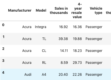
An original data frame with categorical features

First, we select all the columns that are categorical which are those with the data type = ‘object’, creating a data frame subset named ‘dfo’. Next, we concatenate the original data frame df while dropping those columns selected in the dfo, df.drop(dfo,axis=1), with the pandas.get_dummies(dfo)command, creating only indicator columns for the selected object data type columns and collating it with other numeric data frame columns.

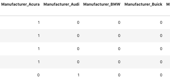
Dummies now added to the data frame with column name such as ‘Manufacturer_’

We perform this conversion regardless of the type of machine learning model we plan on developing because it allows a standardized data set for model development and further data manipulation should our planned approach not provide excellent results in the first pass. Pre-processing is the concept of standardizing your model development dataset.

2. Standardize the magnitude of numeric features

This is applied in situations where you have differences in the magnitude of numeric features. This would also be the juncture where other numeric translation would be applied to meet some scientific assumptions about the feature, such as accounting for atmospheric attenuation in satellite imagery data. However, you do not pass your dummy aka indicator features to the scaler; they do not need to be scaled as they as are boolean representations of categorical features.

Many machine learning algorithms objective functions are based on the assumption that the variables have mean of zero and have variance in the same order of magnitude of one, think L1 and L2 regularization. If the development features are not standardized then the larger magnitude features may dominate the objective function and further may spuriously reduce the impact of other features in the model.

Here is an example, the below data is also from the automobile sales dataset. You can see from the distribution plots for each feature that they vary in magnitude.

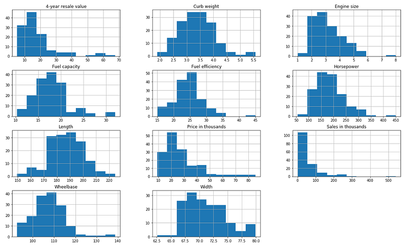
Numeric Features of differing magnitudes

When applying a scaler transformation we must save the scaler and apply the same transformation to the testing data subset. Therefore we apply it in two steps, first defining the scaler based on the mean and standard deviation of the training data and then applying that scaler to each the training and testing sets.

3. Split the data into training and testing subsets

Implementing a data subset approach with a train and test split with a 70/30 or 80/20 split is the general rule for an effective holdout test data for model validation. Review the code snippet and the other considerations below on splitting the model development data set into training and testing subsets.

4. Apply the standard scaler to the testing set

Before applying the scaler we split our dataset into training and testing dataset subsets so we can have a blind hold out sample in the testing set for model evaluation. It would also be appropriate to apply the standard data scaler to the entire data set and then split into test and train subsets afterward. It’s a matter of preference as to which comes first, just ensure the same adjustments applied to the training data are also carried through on the testing data.

Other Considerations in training data development

If you have time series data be sure to consider how to appropriately split your data into training and testing data for your optimal model outcome. Most likely you’re looking to forecast, and your testing subset should probably consist of the time most recent to the expected forecast or for the same period in a different year, or something logical for your particular data.

Additionally, if your data needs to be stratified during the testing and training data split, such as in our example if we considered European carmakers to be different strata then American carmakers we would have included the argument stratify=country in the train_test_split command.

In upcoming articles, I’ll cover machine learning model fitting and model review. Stay in touch by following me on Medium or Twitter. To receive updates about the Data Science Method or Data Science Professional Development Sign up here.