Month: February 2019

Article originally posted on Data Science Central. Visit Data Science Central

Introduction :

Web scraping or crawling is the process of extracting data from any website. The data does not necessarily have to be in the form of text, it could be images, tables, audio or video. It requires downloading and parsing the HTML code in order to scrape the data that you require.

Since data is growing at a fast clip on the web, it is not possible to manually copy and paste it. At times, it is not possible for technical reasons. In any case, web scraping and crawling enables this process of fetching the data in an easy and automated fashion. As it is automated, there’s no upper limit to how much data you can extract. In other words, you can extract large quantities of data from disparate sources.

Data has always been important but of late, businesses have begun to use data in order to make business decisions. As businesses rely heavily on data for decision making, web scraping has, in turn, grown in significance. However, as data needs to be collated from different sources, it is even more important to leverage web scraping as it can make this entire exercise quite easy and hassle-free.  

As information is scattered all over the digital space in the form of news, social media posts, images on Instagram, articles, e-commerce sites etc., web scraping is the most efficient way to keep an eye on the big picture and derive business insights that can propel your enterprise. In this context, java web scraping/crawling libraries can come in quite handy. Here’s a list of best java web scraping/crawling libraries which can help you to crawl and scrape the data you want from the Internet.

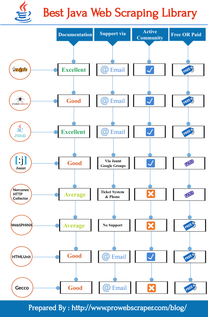
1. Apache Nutch

Apache Nutch is one of the most efficient and popular open source web crawler software projects. It’s great to use because it offers varied extensible interfaces such as Parse, Index and Scoring Filter’s custom implementations such as Apache Tika for parsing. Moreover, it is also possible to use pluggable indexing for Apache Solr, Elastic Search etc.

Pros:

• Highly scalable and relatively feature rich crawler.
• Features like politeness, which obeys robots.txt rules.
• Robust and scalable – Nutch can run on a cluster of up to 100 machines.

Resources:

• Download Apache Nutch
• Learn More: Apache Nutch – Step by Step

2. StormCrawler

StormCrawler stands out as it serves a library and collection of resources that developers can use for building their own crawlers. StormCrawler is also preferred by many for use cases in which the URL to fetch and parse come as streams. However, you can also use it for large scale recursive crawls particularly where low latency is needed.

Pros:

• scalable
• resilient
• low latency
• easy to extend
• polite yet efficient

Resources:

• Download StormCrawler
• Learn More: Getting Started with StormCrawler

3. Jsoup

jsoup is great as a Java library which helps you navigate the real-world HTML. Developers love it because offers quite a convenient API for extracting and manipulating data, making use of the best of DOM, CSS and jquery-like methods.

Pros:

• Fully supports CSS selectors
• Sanitize HTML
• Built-in proxy support
• Provides a slick API to traverse the HTML DOM tree to get the elements of interest.

Resources:

• Download Jsoup
• Learn More: Jsoup HTML parser – Tutorial & examples

4. Jaunt

Jaunt is a unique Java library that helps you in processes pertaining to web scraping, web automation and JSON querying. When it comes to a browser, it does provide web scraping functionality, access to DOM, and control over each HTTP Request/Response but does not support JavaScript. Since Jaunt is a commercial library, it offers diverse kinds of versions, paid as well as free for a monthly download.

Pros:

• The library provides a fast, ultra-light headless browser
• Web pagination discovery
• Customizable caching & content handlers

Resources :

• Download Jaunt
• Learn More: Jaunt Web Scraping Tutorial – Quickstart

5. Norconex HTTP Collector

If you are looking for open source web crawlers related to enterprise needs, Norconex is what you need.

Norconex is a great tool because it enables you to crawl any kind of web content that you need. You can use it as you wish- as a full-featured collector or embed it in your own application. Moreover, it works well on any operating system. It can crawl millions of pages on a single server of median capacity.

Pros:

• Highly scalable – Can crawl millions on a single server of average capacity
• OCR support on images and PDFs
• Configurable crawling speed
• Language detection

Resources:

• Download Norconex HTTP Collector
• Learn More: Getting Started with Norconex HTTP Collector

6. WebSPHINX

WebSPHINX (Website-Specific Processors for HTML INformation eXtraction) is an excellent tool as a Java class library and interactive development environment for web crawlers. WebSPHINX comprises two main parts: the Crawler Workbench and the WebSPHINX class library.

Pros:

• Provide a graphical user interface that lets you configure and control a customizable web crawler

Resources:

• Download WebSPHINX
• Learn More: Crawling web pages with WebSPHINX

7. HtmlUnit

HtmlUnit is a headless web browser written in Java.

It’s a great tool because it allows high-level manipulation of websites from other Java code, including filling and submitting forms and clicking hyperlinks.

It has also got considerable JavaScript support which continues to improve. It is also equipped to work even with the most complex AJAX libraries, simulating Chrome, Firefox or Internet Explorer depending on the configuration used. It is mostly made use of when it comes to testing purposes in order to fetch information from websites.

Pros:

• Provides high-level API, taking away lower-level details away from the user.
• It can be configured to simulate a specific Browser.

Resources:

• Download HtmlUnit
• Learn More: Web Scraping with Java and HtmlUnit

8. Gecco

Gecco is also a hassle-free lightweight web crawler developed with Java language. Gecco framework is preferred for its remarkable scalability. The framework is based on the principle of open and close design, the provision to modify the closure and the expansion of open.

Pros:

• Support for asynchronous Ajax requests in the page
• Support the download proxy server randomly selected
• Using Redis to realize distributed crawling

Resources:  

• Download Gecco
• Learn More: Teach you to use java crawler gecco to grab all JD product information (1)

Conclusion :

As the applications of web scraping grow, the use of Java web scraping libraries is also set to accelerate. Since there are various libraries, and each one has its own unique features, it will require some study on the part of the end user.  However, it will also depend on the respective needs of different end users which will determine which tool would suit better. Once the needs are clear, it would be possible to leverage these tools and power your web scraping endeavours in order to gain a competitive advantage!

Article originally posted on InfoQ. Visit InfoQ

Article originally posted on InfoQ. Visit InfoQ

Article originally posted on InfoQ. Visit InfoQ

According to a paper by a few Google researchers, speculative vulnerabilities currently defeat all programming-language-level means of enforcing information confidentiality. This would not be just an incidental property of how we build our systems, rather the result of wrong mental models that led us to trade security for performance without knowing it.

Our paper shows these leaks are not only design flaws, but are in fact foundational, at the very base of theoretical computation.

Information confidentiality is a highly desirable property of a system that should be enforced at different levels of abstractions, from the hardware up to the programming language.

Programming languages provide a varying number of provisions to guarantee confidential information is not leaked. For example, in many mainstream languages, the type system is designed to rule out a number of dangerous behaviours which could put at risk integrity, confidentiality, and availability. One of the most significant properties type systems attempt to enforce is memory-safety, often the culprit behind many vulnerabilities, and a lot of research and effort have gone into building languages in such a way they can be trusted not to do unexpected things. Spectre has changed all that, according to Google researchers.

Spectre allows for information to be leaked from computations that should have never happened according to the architectural semantics of the processor. […] This puts arbitrary in-memory data at risk, even data “at rest” that is not currently involved in computations and was previously considered safe from side-channel attacks.

To clarify this claim, the researchers defined a formal model of micro-architectural side-channels used to define an association between a processor’s architectural states, i.e. the view of the processor that is visible to a program, and its micro-states, the CPU’s internal states below the abstraction exposed to programming languages. This association shows how many correct micro-states may map to a single architectural state.

For example, when a CPU uses a cache or a branch predictor, the timings associated with a given operation will vary depending on the CPU micro-state, e.g., the data may be already available in the cache or needing to be fetched from memory, but all possible micro-states will correspond to the same architectural state, e.g. use a piece of information. Furthermore, the researchers define a technique to amplify timing differences and make them easily detectable, which becomes the base for the construction of a universal “read gadget”, a sort of “out-of-bounds memory reader” giving access to all addressable memory.

According to the researchers, such a universal read gadget may be built for any programming language –even if it is not necessarily a trivial task– leveraging a number of language constructs or features that they have shown to be vulnerable using their model. Those include indexed data structures with dynamic bounds checks; variadic arguments; dispatch loops; call stack; switch statements, and more.

As a conclusion, the community is facing three major challenges: discovering micro-architectural side-channels; understanding how programs can manipulate micro-states; and how to mitigate those vulnerabilities.

Mitigating vulnerabilities is perhaps the most challenging of all, since efficient software mitigations needed for extant hardware seem to be in their infancy, and hardware mitigation for future designs is a completely open design problem.

While not reassuring, the paper makes for a quite dense read full of insights into how our mental computation model diverge from real computations happening in CPUs.

Article originally posted on Data Science Central. Visit Data Science Central

Monday newsletter published by Data Science Central. Previous editions can be found here. The contribution flagged with a + is our selection for the picture of the week. To subscribe, follow this link.  

Featured Resources and Technical Contributions 

• New Perspectives on Statistical Distributions and Deep Learning +
• Python machine learning libraries 
• Can you be a Data Scientist without coding? 
• Visualizing New York City WiFi Access with K-Means Clustering 
• Tutorial: Statistical Tests of Hypothesis 
• Image Recognition with Keras: Convolutional Neural Networks 
• Math You Don’t Need to Know for Machine Learning 
• Top takeaways from R Studio conf 2019 
• How to Configure the Number of Layers and Nodes in a Neural Network 

Featured Articles and Forum Questions

• How to Stabilize Data Systems, to Avoid Decay in Model Performance 
• Should you Add your Coursera, Udacity, or DataCamp Training to your Resume? 
• Should CEOs Learn To Code? Yes! 
• Top 7 Data Science Use Cases in Travel 
• From Optimization to Prescriptive Analytics 
• How Big Data and Education Can Work Together to Help Students Thrive 
• Data Anonymisation Software – Static vs Interactive 
• Question: Will humans become to AI what dogs are to humans now? 
• And Monty Hall Went Bayesian… 

Picture of the Week

Source for picture: contribution marked with a + 

To make sure you keep getting these emails, please add  mail@newsletter.datasciencecentral.com to your address book or whitelist us. To subscribe, click here. Follow us: Twitter | Facebook.

  Hire a Data Scientist | Search DSC | Find a Job | Post a Blog | Ask a Question

Article originally posted on InfoQ. Visit InfoQ

Palantir, the creators of TSLint, recently announced the deprecation of TSLint, putting their support behind typescript-eslint to consolidate efforts behind one unified linting solution for TypeScript users.

Discussions between the TypeScript team, ESLint team, and TSLint team have been ongoing. In January the TypeScript team announced plans to adopt ESLint. TypeScript program manager Daniel Rossenwasser explains:

The most frequent theme we heard from users was that the linting experience left much to be desired. Since part of our team is dedicated to editing experiences in JavaScript, our editor team set out to add support for both TSLint and ESLint. However, we noticed that there were a few architectural issues with the way TSLint rules operate that impacted performance.

Upon hearing this news, the ESLint team announced the separation of TypeScript-specific ESLint efforts into a separate project to be led by Nrwl software engineer James Henry:

James Henry, who has long been the driving force behind TypeScript compatibility for ESLint, has started the typescript-eslint project as a centralized repository for all things related to TypeScript ESLint compatibility. This will be the new home of the TypeScript parser, eslint-plugin-typescript, and any other utilities that will make the TypeScript ESLint experience as seamless as possible.

This separation will allow for ESLint compatibility, while maintaining a separate focus on TypeScript specific needs. As explained by the ESLint team:

While the ESLint team won’t be formally involved in the new project, we are fully supportive of James’ efforts and will be keeping lines of communication open to ensure the best ESLint experience for TypeScript developers.

The TSLint team at Palantir was very much aware of the compatibility challenges with ESLint and TSLint. After the TypeScript team explained the goal in their roadmap to help converge the TypeScript and JavaScript developer experience converge, Palantir’s TSLint team met with the TypeScript team to discuss the future of TypeScript linting and decided to back the efforts of typescript-eslint

Palantir’s goals for supporting the TSLint community with a smooth transition to ESLint include:

• Support and documentation for authoring ESLint rules in TypeScript
• Testing infrastructure in typescript-eslint
• Semantic, type-checker-based rules

Once Palantir considers ESLint feature-complete, TSLint will get deprecated. Before that date, Palantir pledges to continue TSLint support for new TypeScript releases. Once compatibility is reached, plans include a TSLint to ESLint compatibility package to make ESLint work as a drop-in replacement for the TSLint rule set.

typescript-eslint is an open source monorepo for tooling to enable ESLint to support TypeScript and is available under the New BSD License and supported by the JS Foundation. Contributions are welcome via the typescript-eslint GitHub project.

Article originally posted on InfoQ. Visit InfoQ

Preferring frameworks or libraries is somewhat controversial, Frans van Buul, commercial director and evangelist at AxonIQ, the company behind Axon Framework, writes in a recent blog post. Many argue in the favour of libraries but Van Buul thinks that a framework can be very valuable when building business applications. He believes this to be especially true for applications using the architectural concepts found in Axon — CQRS, DDD and event sourcing.

A library is defined by Van Buul as a body of code, consisting of classes and functions, which is used by an application, but without being part of that application. An application interacts with the library by doing function or method calls into the library. He defines a framework as a special kind of library where interaction is the other way around, an application now implements interfaces in the framework, or use annotations from it. During execution the framework invokes application code; using a library it’s the other way around.

Creating an application without using a framework is for Van Buul somewhat of a mirage, claiming that even if you just use the Java platform, you are also using a framework. He points out that the Java platform is an abstraction over the operating system and the machine and that the platform is invoking the application code. He also notes that most business applications have a web-based interface and use an abstraction layer to create entry points into the application — meaning a framework is used.

Reasoning about the advantages of using a framework, Van Buul assumes that CQRS, DDD and event sourcing are requirements. His first argument is that it allows developers to focus on the business domain instead of on infrastructure. He believes that in practice the alternative is not to use a library, but to build your own framework. This can in the end be a very complex task and force developers to spend a lot of time creating the framework. He claims that this will both increase the risk and the cost and strongly advices against doing this. He refers to Greg Young, who coined the term CQRS, and his presentation at DDD Europe 2016 where he advised:

Don’t write a cqrs framework

Peter Kummins sees frameworks as one of the largest anti-patterns in system development, arguing that they are hard to learn and increase a project’s complexity and dependencies. He claims that software should be developed using the least amount of complexity, using fundamental tools that have been and will be around for the next 20 years, and prefers using core language solutions and small abstractions or helper libraries before general libraries and frameworks.

Kummins’ main reasons for not using frameworks include that they:

• are hard to learn, and this knowledge is generally useless
• limit your scope of creativity
• increase a project’s complexity
• go out of business

Mathias Verraes agrees with the definition of a framework and refers to the mnemonic:

A library is something your code calls, a framework calls your code

He argues against frameworks, claiming that the cost of a boilerplate in a system that is 10 years old is negligible, compared to the cost of badly understood, obsolete or plain wrong abstractions. His recommendation is therefore to use frameworks only for applications with a short development lifespan, and to avoid frameworks for systems you intend to keep for multiple years.

Tomas Petricek uses the same framework definition and argues that the biggest and most obvious problem with frameworks is that they cannot be composed. When using two frameworks there is commonly no way to fit one of them into the other; when using two libraries this is easily done. He also notes that frameworks are hard to explore and affect the way you code.

Petricek refers to functional library design principles and points out that one way of getting away from frameworks and callbacks is to use asynchronous workflows and an event-based programming model. Instead of writing abstract or virtual methods that need to be implemented, events are exposed and triggered when an operation needs to be done. He notes that with this model, although we are not in full control since we don’t know when an event is triggered, we are in control after that. Reversing the control this way makes it possible to use composable libraries instead of frameworks and to choose which library to use for a specific part of a problem.

In conclusion, Van Buul notes that one argument for favouring libraries is that they are more flexible, but claims that this depends on the framework. For a framework closed for extension it’s probably true, but for an open source framework with core concepts defined as open interfaces, he believes it can be as flexible as a library.

Article originally posted on Data Science Central. Visit Data Science Central

Whether you can call yourself a data scientist if you can’t code is as hotly debated as Brexit. Type the question “Can you be a Data Scientist without coding?” into Google and you’ll get a hundred different answers. The opinion will vary wildly depending on whether the author is a coder, or a non-coder. Search the job listings, and you won’t find a definitive answer there either. A Glassdoor survey on the skills required for data science job postings showed that for every 10 job postings, nine required at least Python, R, and/or SQL skills. So while coding is a “common” requirement, is it a necessity in today’s ever changing machine learning landscape?

Rather than fill the internet with yet another opinion (as I am not a coder, my opinion would be quite biased), I thought I would perform a little meta analysis. For this post, I pooled data from about sixty different sources, to uncover current thinking on what is quite a debatable topic. You won’t find all sources listed below, as I have no wish to bloat out a blog post with a dissertation worthy reference list. But my methodology was simply to type the question into Google, and click on the first  25 search results for each category (Opinion Sites/Business/*.edu/). I figured that would get me the current/popular thoughts. Any “Wiki” style sites were filtered out (as it would be difficult to ascertain whether those posts were the opinions of a business person, academic, or other), as were multiple posts from the same site.

Can you be a Data Scientist without coding? The NO camp

Opinion sites (like newspapers and magazines) and bloggers are firmly split down the middle of the “coding or no coding” debate. The analytics dude Eric Hulbert sums up the answer to the question “Can you be a data scientist without knowing how to code?” with a single word “Nope” (although he does go on to explain the “nuances” of that statement). Rachael Tatman, writing on freeCodeCamp states that every data scientist should be able to “write code for statistical computing and machine learning.”  Ronald Van Loon agrees, giving a rather lengthy list of required technical skills including knowledge of programming languages like Python, Perl, C/C++, SQL and Java plus expertise in tools like SAS, Hadoop, Spark, Hive, Pig.

Also in the “No” camp is the Executive recruiting company Burtch Works, which lists the following “Must-Have Skills that employers are looking for: Python coding (along with Java, Perl, or C/C++) and machine learning. Experience with Hadoop, Hive, or Pig is a “strong selling point.”

In education, many university websites tend to be planted firmly in the “no” camp, but many of the articles are outdated when you consider that DS has only been a “thing” for a decade. For example, this article on Columbia University’s website (from 2013) is titled “Statistics is the least important part of data science”.

Ouch.

With today’s ever changing DS realm, one could argue that statistics is one of the most important parts of data science. In 2018, it’s certainly not the least important.

Georgetown university’s Advice to Future Data Scientists also stands firmly in the No camp; “Write Code, Any Code.” That said, further down the page the article states “Focus on what you’re good at. Not everyone is a programmer. Not everyone is a statistician…Whatever interests you, whatever talent you have, augment your assignments with that.” At first, that sounds like you might be able to get away with just being a statistician. But notice the word augment  in there: they are still telling you to code, code, code–and augment it with other things (like programming or statistics).

Can you be a Data Scientist without coding? The YES camp

Blogger Tom Wentworth’s opinion, writing for Rapid Miner: “Yes, you can do real data science without writing code. ” Perhaps the most important question here is: why don’t you need to be able to code to be a data scientist? Many people give solid reasons why. Here are a few of the more popular:

• Common algorithms are already known, coded and optimized.
• Explicit coding is being replaced with drag-and-drop interfaces, like Trifacta and Tableau.
• Data science is becoming more automated with options like Google’s Cloud AutoML or DataRobot, both of which help you to find the right algorithm. Google promises that you can “Train high-quality custom machine learning models with minimum effort and machine learning expertise.”
• Talking of automation, the Google Duplex demo hinted at the future of AI. The future data scientist might simply be having a conversation with a machine, rather than coding one.

Also in the Yes camp is Dana Parks’ 2017 dissertation titled Defining Data Science and Data Scientist. Parks’ dissertation is an attempt to “[establish] set guidelines on how data science is performed and measured. Important findings include that the “Ability to write code using Java, C, C++ and HTML [is] common among practitioners.” However, “The academic community did not consider this skill as necessary for data scientists. ” This is a fairly up to date paper, and a much more in depth analysis of current thinking on the coding debate that I can squeeze into a blog post. Therefore, it’s worth a read (and is available in it’s entirety here).

Can you be a Data Scientist without coding? The “Maybe” camp

Bob Violino offers little hope for the non-coder: “top-notch data scientists know how to write code”. While that means you can’t rise to the very top without knowing code, you can probably still get a foot in the door. And as you make your way up the ranks, Violino offers this nugget of advice: “If a data scientist doesn’t understand how to code, it helps to be surrounded by people who do [like a developer].”

While it doesn’t explicitly state much about the requirement of coding, this 2017 article on the University of Notre Dame website states that “employers are increasingly valuing data scientists who can take on more responsibility beyond their coding or technical duties.” Even more interesting is the trend for higher salaries to be linked not to coding expertise but to the amount of time spent in meetings. The top salaries for data scientists tend to go to those who spend more than 20 hours a week in meetings. 

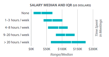
Image:  2017 Data Scientist Salary Survey from O’Reilly, posted on the University of Notre Dame website.

If that sounds like you might want to brush up on your interpersonal relationship skills instead of coding, don’t snap your laptop shut yet. This University of Wisconsin article notes that, “the highest data scientist salaries belong to those who code four to eight hours per week; the lowest salaries belong to those who don’t code at all.” The biggest coding factor that affects salary? Knowledge of Apache Hadoop will affect your salary by 8%. Before you get alarmed though, bear in mind that a lot of institutions are merely using statistics to sell their wares. The University of Wisconsin notes that “only a data science masters degree will give you the precise education you need to be ready for a career in data science,” placing them firmly in the “Maybe” camp.

Conclusion

There are strong voices on both sides of the data science and coding debate. Perhaps the two antipodean camps are a product of the recency of data science and the lack of a solid definition of what exactly a “Data Scientist” is. Trying to pin down a solid definition for “Data Scientist” is like pinning down a universal definition for “expert”. John D Cook attempts to clarify the DS definition by splitting data science into two realms: The statistician who can code (which cook calls “Type A”) and the strong coders / software engineers who know a little statistics (“Type B”).

The definition is hard to pin down and seems to be ever changing. Ten years ago, very few people were using the job title “data scientist”, and there wasn’t such a thing as a “data science” degree. The internet was still in its infancy and coding was a must. Nowadays, with many algorithms already worked out and universally available online, coding doesn’t seem to be a “must” any more. 

If you’re a non-coder then, what do you need? Meta S. Brown, author of Data Mining for Dummies, wrote in a Forbes article that “…a person with a Bachelor’s degree, some worthwhile industry experience, and skills in statistics or programming…has a chance to get into the data science game.” So if you decide you’re not a coder, and you want an alternate path to becoming a data scientist, then statistics is the way to go.

My two cents? Ignore (for the most part) the confusing “advice” dished out on the internet, and simply do what you love. If statistics is your thing, then study that and forget coding (for now). Like coding? Forget the statistics (for now) and code your happy heart out.

References

• Can you be a data scientist without coding?
• You Can Get A Data Analytics Job Without A Masters In Data Science
• Data engineers vs. data scientists
• Scaling Data Science Without Data Scientists
• Must-Have Skills You Need to Become a Data Scientist
• 12 Mistakes that Data Scientists Make and How to Avoid Them
• Statistics is the least important part of data science
• Advice to Future Data Scientists: Write Code, Any Code
• Defining Data Science and Data Scientist
• A rose by any other name: Data science etc.
• Data Scientist Personas: What Skills Do They Have and How Much Do They Make?
• How Much Is a Data Scientist’s Salary?

Article originally posted on InfoQ. Visit InfoQ

At BlueHat IL 2019, Microsoft engineer Matt Miller described how the software vulnerability landscape has evolved over the last 20+ years and the approach Microsoft has been taking to mitigate threats. Interestingly, among the major culprits of security bugs, says Miller, are memory safety issues, which account for 70% of total security bugs Microsoft has patched.

The analysis of the root causes of security vulnerabilities is the first step that can be taken to define a correct approach to risk mitigation, according to Miller.

What’s noteworthy here is that at a macro scale, going all the way back to 2006, memory safety issues remain the most common kind in this category of vulnerabilities that we’re looking at. About 70% of the vulnerabilities that are addressed through a security update each year are related to a memory safety issue.

Now, memory safety is a big category, including several kinds of issues, from stack and heap corruption to use after deallocation, uninitialized memory access, and so on. Analyzing the evolution of those sub-categories, Miller points out that stack corruptions went from contributing a non-trivial proportion of vulnerabilities to being almost non existent. Similarly, usage after deallocation accounted for more than 50% of vulnerabilities in 2013-2015 due to Web browser bugs and then decreased significantly thanks to the use of garbage collection. On the other hand, heap out-of-bounds read, type confusion, and uninitialized access have increased across the last few years.

Moving from discovered vulnerabilities to actually exploited vulnerabilities, Miller shows a slightly different picture, where accessing memory after freeing it and heap corruption are the most exploited kind of vulnerabilities.

The reason why this is interesting is because this provides us hints in terms of what are the types of vulnerabilities that may be easier or more preferred by attackers in terms of going and trying to exploit them.

Knowing where security issues arise and what kind of vulnerabilities attackers prefer provides does not actively contribute to reducing vulnerabilities of a software system, though. For this, a number of challenges must be overcome, says Miller.

We still do see many of the making some of the same mistakes that were made 10 years ago.

This has to do with a number of reasons, including the complexities of dealing with undefined behaviour in languages like C and C++, lack of tools or training, or even the fact that software is increasingly developed at different groups following different security policies and standards.

Another area where progress can be made is finding ways to break exploitation techniques. Indeed, exploits tend to use the same general pattern where you leverage a vulnerability to read or write from an arbitrary memory location and get the chance to discover interesting things about the program, such as which DLLs it uses and so on. Using that information, you set up a malicious payload that you use to try to hijack the control flow of the program, such as by corrupting a function pointer, or a virtual table pointer, and so on.

Summing it all up, says Miller, the most promising approach to reducing vulnerabilities is aiming for a more radical shift where you:

• Make unsafe code safer by eliminating common classes of memory safety vulnerabilities.
• Use safer languages, such as C# or Rust, or improve existing languages like C++.
• Improve development process and tools, including compiler autofix and alike.

There is a lot more in Miller’s talk that can be covered here. Do not miss his talk recording to get the full detail.

Article originally posted on Data Science Central. Visit Data Science Central

In this data science article, emphasis is placed on science, not just on data. State-of-the art material is presented in simple English, from multiple perspectives: applications, theoretical research asking more questions than it answers, scientific computing, machine learning, and algorithms. I attempt here to lay the foundations of a new statistical technology, hoping that it will plant the seeds for further research on a topic with a broad range of potential applications. 

1. Introduction

In a previous article (see here) I attempted to approximate a random variable representing real data, by a weighted sum of simple kernels such as uniformly and independently, identically distributed random variables. The purpose was to build Taylor-like series approximations to more complex models (each term in the series being a random variable), to

• avoid over-fitting,
• approximate any empirical distribution (the inverse of the percentiles function) attached to real data, with  the distribution attached to the first few terms the weighted sum representation
• easily compute data-driven confidence intervals regardless of the underlying distribution,
• derive simple tests of hypothesis,
• perform model reduction, 
• optimize data binning to facilitate feature selection, and to improve visualizations of histograms
• create perfect histograms,
• build simple density estimators,
• perform interpolations, extrapolations, or predictive analytics
• perform clustering and detect the number of clusters.

Why I’ve found very interesting properties about stable distributions during this research project in my previous article, I could not come up with a solution to solve all these problems. The fact is that these weighed sums would usually converge (in distribution) to a normal distribution if the weights did not decay too fast — a consequence of the central limit theorem. And even if using uniform kernels (as opposed to Gaussian ones) with fast-decaying weights, it would converge to an almost symmetrical, Gaussian-like distribution. In short, very few real-life data sets could be approximated by this type of modeling.

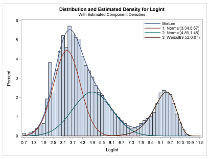
Source for picture: SAS blog

I also tried with independently but NOT identically distributed kernels, and again, failed to make any progress. By not identically distributed kernels, I mean basic random variables from a same family, say with a uniform or Gaussian distribution, but with parameters (mean and variance) that are different for each term in the weighted sum. The reason being that sums of Gaussian’s, even with different parameters, are still Gaussian, and sums of Uniform’s end up being Gaussian too unless the weights decay fast enough. Details about why this is happening are provided in the appendix. 

Now, in this article, starting in the next section, I offer a full solution, using mixtures rather than sums. The possibilities are endless. 

2. Approximations Using Mixture Models

The problem is specified as follows. You have an univariate random variable Y that represents any of your quantitative features in your data set, and you want to approximate it by a mixture of n elementary independent random variables called kernels and denoted as X(n, k) for k = 1, …, n, with decreasing probability weights p(n, k) that converge to zero. The approximation of Y based on the first n kernels, is denoted as Y(n). By approximation, we mean that the data-generated empirical distribution of Y is well approximated by the known, theoretical distribution of Y(n) and that as n tends to infinity, both become identical (hopefully).

Moving forward, N denotes your sample size, that is the number of observations; N can be be very large, even infinite, but you want to keep n as small as possible. Generalizations to the multivariate case is possible but not covered in this article. The theoretical version of this consists in approximating any known statistical distribution (not just empirical distributions derived from data sets) by a small mixture of elementary (also called atomic) kernels.

In statistical notation, we have:

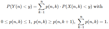
We also want Y(n) to converge to Y, in distribution, as n tends to infinity. This implies that for large n, the weights p(n, k) must tend to zero as k tends to infinity. 

The error term

There are various ways to define the distance between two distributions, say Y(n) and Y. See here for details; one of the most popular ones is the Kolmogorov-Smirnov metric. Regardless of the metric used, the error term is denoted as E(n) = ||Y – Y|(n)|. Of course, the problem, for a given value of n, is to minimize E(n). As n tends to infinity, by carefully choosing the parameters in the model (that is, the weights, as well the the means and variances of the kernels,)  the error E(n) is supposed to converge to 0. Note that the kernels are independent random variables, but not identically distributed: a mix of kernels with different means and variances is not only allowed, but necessary to solve this optimization problem.

Kernels and model parameters

Besides the weights, the other parameters of the models are the parameters attached to each kernel X(n, k). Typically, each kernel X(n, k) is characterized by two parameters: a(n, k) and b(n, k). In the case of Gaussian kernels, a(n, k) is the mean and b(n, k) is the variance; b(n, k) is set to 1. In the case of Uniform kernels with Y taking on positive values, a(n, k) is the lower bound of the support interval, while b(n, k) is the upper bound; in this case, since we want the support domains to form a partition of the set of positive real numbers (the set of potential observations), we use, for any fixed value of n,  a(n, 1) = 0 and  b(n, k) = a(n, k+1).

Finally,the various kernels should be re-arranged (sorted) in such a way that X(n, 1) always has the highest weight attached to it, followed by X(n, 2), X(n, 3) and so on. The methodology can also be adapted to discrete observations and distributions, as we will discuss later in this article. 

Algorithms to find the optimum parameters 

The goal is to find optimum model parameters, for a specific n, to minimize the error E(n). And then try bigger and bigger values of n, until the error is small enough. This can be accomplished in various ways.

The solution consists in computing the derivatives of E(n) with respect to all the model parameters, and then finding the roots (parameter values that make the derivatives vanish, see for instance this article.) For a specific value of n, you will have to solve a non-linear system of m equations with m parameters. In the case of Gaussian kernels, m = 2n. For uniform kernels, m = 2n + 1 (n weights, n interval lower bounds, plus upper bound for the rightmost interval.) No exact solution can be found, so you need to use an iterative algorithm. Potential modern techniques used to solve this kind of problem include:

• Swarm gradient optimization
• EM algorithm
• Stochastic gradient descent

You can also use Monte-Carlo simulations, however here you face the curse of dimensionality, the dimension being the number m of parameters in your model. In short, even for n as small as n = 4 (that is, m = 8), you will need to test trillions of randomly sampled parameter values (m-dimensional vectors) to get a solution close enough to the optimum, assuming that you use raw Monte-Carlo techniques. The speed of convergence is an exponential function of m. Huge improvements to this method are discussed later in this section, using some kind of step-wise algorithm to find local optima, reducing it to a 2-dimensional problem. By contrast, speed of convergence is quadratic for gradient-based methods, if E(n) is convex in the parameter space. Note that here, E(n) may not be convex though.  

Convergence and uniqueness of solution 

In theory, both convergence and the fact that there is only one global optimum, are guaranteed. It is easy to see that under the constrained imposed here on the model parameters, two different mixture models must have two distinct distributions. In the case of Uniform kernels, this is because the support domains of the kernels form a partition, and are thus disjoint. In the case of Gaussian kernels, as long as each kernel has a different mean, no two mixtures can have the same distribution: the proof is left as an exercise. To put it differently, any relatively well behaved statistical distribution is uniquely characterized by its set of parameters associated with its mixture decomposition. When using Gaussian kernels, this is equivalent to the fact that any infinitely differentiable density function is uniquely characterized by its coefficients in its Taylor series expansion. This is discussed in the appendix.

The fact that under certain conditions, some of the optimization algorithms described in the previous subsection, converge to the global optimum, is more difficult to establish. It is always the case with the highly inefficient Monte Carlo simulations. In that case, the proof is pretty simple and proceeds as follows

• Consider the discrete case where Y takes only on positive integer values (for example, your observations consist of counts,) and use the discrete Uniform kernel.
• In that case, the solution will converge to a mixture model where each kernel is a binomial random variable, and its associate weight is the frequency of the count in question, in your observed data. This is actually the global optimum, with E(n) converging to 0 as n tends to infinity. 
• Continuous distributions can be approximated by discrete distributions after proper re-scaling. For instance, a Gaussian distribution can be perfectly approximated by sequences of increasingly granular binomial distributions. Thus, the convergence to a global optimum, can be derived from the convergence obtained for the discrete approximations. 

The stopping rule, that is, deciding when n is large enough, is based on how fast E(n) continue to improve as n increases. Initially, for small but increasing values of n, E(n) will drop sharply, but for some value of n usually between n = 3 and n = 10, improvements will start to taper off, with E(n) very slowing converging to 0. If you plot E(n) versus n, the curve will exhibit an elbow, and you can decide to stop at the elbow. See the elbow rule here. 

Finally, let us denote as a(k) the limit of a(n, k) as n tends to infinity; b(k) and p(k) are defined in a similar manner. Keep in mind that the kernels must be ordered by decreasing value of their associated weights. In the continuous case, a theoretical question is whether or not these limits exist. With Uniform kernels, p(n, k), as well as b(n, k) – a(n, k), that is, the length of the k-th interval, should both converge to 0, regardless of k, as n tends to infinity.  The limiting quotient represents the value of Y‘s density at the point covered by the interval in question. Also, the sum of p(n, k) over all k‘s, should still be equal to one, at the limit as n tends to infinity. In practice, we are only interested in small values of n, typically much smaller than 20.

Find near-optimum with fast step-wise algorithm

A near optimum may be obtained fairly quickly with small values of n, and in practice this is good enough. To further accelerate the convergence, one can use the following step-wise algorithm, with the Uniform kernel. At iteration n+1, modify only two adjacent kernels that were obtained at iteration n (that is, kernels with adjacent support domains) as follows:

• Increase the upper bound of the left interval, and decrease the lower bound of the right interval accordingly. Or do the other way around. Note that the cumulative density within each interval, before or after modification, is always equal to 1, since we are using uniform kernels.
• Adjust the two weights, but keep the sum of the two weights unchanged.

So in fact you are only modifying two parameters (degrees of freedom is 2.) Pick up the two intervals, as well as the new weights and lower/upper bounds, in such a way as to  minimize E(n+1).

3. Example

Here, I illustrate some of the concepts explained earlier, with an example based on simulated data. The source code and the data is provided so that my experiment can be replicated, and the technical details understood.  The 10,000 data points generated (representing Y) are deviates from a skewed, non-symmetrical negative binomial distribution, taking integer values between 0 and 110. Thus we are dealing with discrete observations and distributions. The kernels have discrete uniform distributions, for instance uniform on {5, 6, 7, 8, 9, 10, 11} or on {41, 42, 43, 44}. The choice of a non-symmetrical target distribution (for Y) is to illustrate the fact that the methodology also works for non-Gaussian target variables, unlike the classic central limit theorem framework applying to sums (rather than mixtures) and where convergence is always towards a Gaussian. Here instead, convergence is towards a simulated negative binomial.   

I tried to find online tools to generate deviates from any statistical distribution, but haven’t found any interesting ones. Instead, I used R to generate the 10,000 deviates, with the following commands:

The first line of code generates the 10,000 deviates from a negative binomial distribution, the second line produces its histogram with 50 bins (see picture below, where the vertical axis represents frequency counts, and the horizontal axis represents values of Y.)  The third line of code exports the data to an output file that will first be aggregated and then used as an input for the script that (1) computes the model parameters, and (2) computes and minimizes the error E(n).

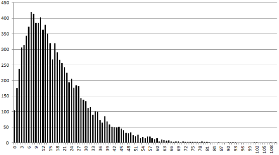
Histogram for the 10,000 deviates (negative binomial distribution) used in our example

Data and source code

The input data set for the script that processes the data, can be found here. It consists of the 10,000 negative binomial deviates (generated with the above R code), and aggregated / sorted by value. For instance, the first entry (104) means that among the 10,000 deviates, 104 of them have a value equal to 0. The second entry (175) means that among the 10,000 deviates, 175 of them have a value equal to 1. And so on.

The script is written in Perl (you are invited to write a Python version) but it is very easy to read and well documented. It illustrates the raw Monte-Carlo simulations with 4 discrete uniform kernels. So it is very inefficient in terms of speed, but easy to understand, with few lines of code. You can find it here. It produced the distribution (mixture of 4 kernels) that approximates the above histogram, see picture below.

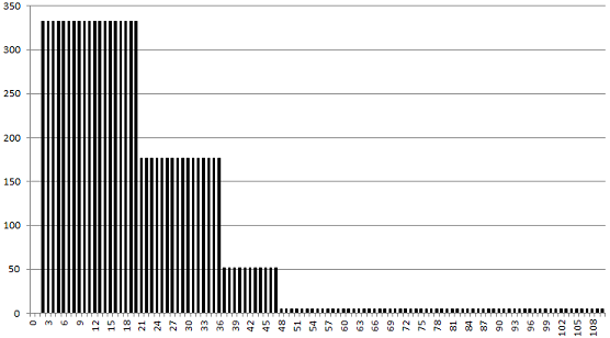
Approximation of above histogram with mixture model, using 4 uniform kernels

Results 

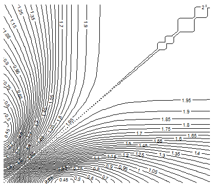
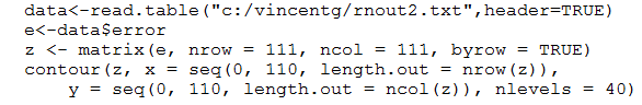
The chart below shows a contour plot for the error E(2), when using n = 2 discrete uniform kernels, that is two intervals, with lower bounds of the first interval displayed on the vertical axis, and upper bounds on the horizontal axis. The upper bound of the second (rightmost) interval was set to the maximum observed value, equal to 110. Ignore the curves above the diagonal; they are just a mirror of the contours below. Outside the kernel intervals, densities were kept to 0. Clearly the best kernel (discrete) intervals to approximate the distribution of Y,  are visually around {1, 2, … , 33}  and {34, …, 110} corresponding to a lower bound of 1, and an upper bound of 33 for the first interval; it yields an error E(2) less than 0.45.

The contour plot below was produced using the contour function in R, using this data set as input, and the following code:

The interesting thing is that the error function E(n), as a function of the mixture model parameters, exhibit large areas of convexity containing the optimum parameters, when n = 2. This means that gradient descent algorithms (adapted to the discrete space here) can be used to find the optimum parameters. These algorithms are far more efficient than Monte-Carlo simulations. 

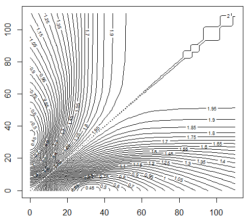
Contour plot showing the area where optimum parameters are located, minimizing E(1)

I haven’t checked if the convexity property still holds in the continuous case, or when you include the weight parameters in the chart, or for higher values of n. It still might, if you use the fast step-wise optimization algorithm described earlier. This could be the best way to go numerically, taking advantage of gradient descent algorithms, and optimizing only a few parameters at a time.

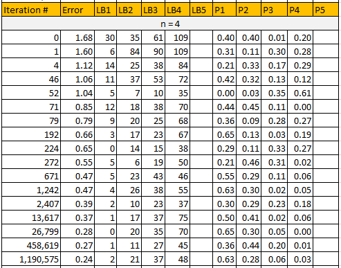
Now I discuss the speed of convergence, and improvements obtained by increasing the number of kernels in the model. Here, optimization was carried via very slow, raw Monte-Carlo simulations. The table below shows the interval lower bounds and weights associated with the discrete uniform kernel, for n = 4, obtained by running 2 million simulations. The upper bound of the rightmost interval was set to the maximum observed value, equal to 110. For any given n, only simulations performing better than all the previous ones, are displayed: in short, these are the records. Using n = 5 does not improve the final error E(n). Low errors with n = 2, 3, and 4 were respectively 0.41, 0.31, and 0.24. They were obtained respectively at iterations 7,662 (n = 2), 96,821 (n = 3) and 1,190,575 (n=4). It shows how slow Monte-Carlo converges, and the fact that the number of required simulations grows exponentially with the dimension n. The Excel spreadsheet, featuring the same table for n = 2, 3, 4, and 5, can be found here.

4. Applications

The methodology proposed here has many potential applications in machine learning and statistical science. These applications were listed in the introduction. Here, I just describe a few of them in more details. 

Optimal binning

These mixtures allow you to automatically create optimum binning of univariate data, with bins of different widths and different sizes. In addition, the optimum number of bins can be detected using the elbow rule described earlier. Optimum binning is useful in several contexts: visualization (to display meaningful histograms), in decision trees, and in feature selection procedures. Some machine learning algorithms, for instance this one (see also here,) rely on features that are not too granular and properly binned, to avoid over-fitting and improve processing time. These mixture models are handy tools to help with this.

Predictive analytics

Since this methodology creates a simple model to fit with your data, you can use that model to predict frequencies, densities, (including perform full density estimation), intensities, or counts attached to unobserved data points, especially if using kernels with infinite support domains, such as Gaussian kernels. It can be used as a regression technique, or for interpolation or extrapolation, or for imputation (assigning a value to a missing data point), all of this without over-fitting. Generalizing this methodology to multivariate data will make it even more useful.

Test of hypothesis and confidence intervals

These mixtures help build data-driven intermediate models, something in-between a basic Gaussian or exponential or whatever fit (depending on the shape of the kernels) and non-parametric empirical distributions. It also comes with core parameters (the model parameters) automatically estimated. Confidence intervals and tests of hypothesis are easy to derive, using the approximate mixture model distribution to determine statistical significance, p-values, or confidence levels, the same way you would with standard, traditional parametric distributions. 

Clustering

Mixture models were invented long ago for clustering purposes, in particular under a Bayesian framework. This is also the case here, and even more so as this methodology gets extended to deal with multivariate data. One advantage is that it can automatically detect the optimum number of clusters thanks to its built-in stopping rule, known as the elbow rule. Taking advantage of convexity properties in the parameter space, to use gradient descent algorithm for optimization, the techniques described in this article could perform unsupervised clustering faster than classical algorithms, and be less computer intensive.   

5. Appendix

We discuss here, from a more theoretical point of view, two fundamental results mentioned earlier. 

Gaussian mixtures uniquely characterize a broad class of distributions 

Let us consider an infinite mixture model with Gaussian kernels, each with a different mean a(k), same variance equal to 1, and weights p(k) that are strictly decreasing. Then the density associated with this mixture is

Two different sets of (a(k), p(k)) will result in two different density functions, thus the representation uniquely characterizes a distribution.  Also, the exponential functions in the sum can be expanded as Taylor series. Thus we have:

Density functions infinitely differentiable at y = 0, can be represented in this way. Convergence issues are beyond the scope of this article.

Weighted sums fail to achieve what mixture models do

It is not possible, using an infinite weighted sum of independent kernels of the same family, with decaying weights converging to zero but not too fast, to represent any arbitrary distribution. This fact was established here in the case where all the kernels have the exact same distribution. It is mostly an application of the central limit theorem. Here we generalize this theorem to kernels from a same family of distributions, but not necessarily identical. By contrast, the opposite is true if you use mixtures instead of weighted sums.

With a weighted sum of Gaussian kernels of various means and variances, we always end up with a Gaussian distribution (see here for explanation.) With Uniform kernels (or any other kernel family) we can prove the result as follows:

• Consider a sum of n kernels from a same family. Say n(1) of them have (almost) the same parameters, another n(2) of them have the same parameters but different from the first group, another n(3) of them have the same parameters but different from the first two groups, and so on, with n = n(1) + n(2) + …
• Let n tends to infinity, with n(1), n(2) and so on also tend to infinity. The weighted sum in each group will converge to Gaussian, by virtue of the central limit theorem.
• The overall sum across all groups will tend to a sum of Gaussian, and thus must be Gaussian. This depends on how fast the weights are decaying. Details about the decaying rate, for the result to be correct, are provided in my previous article. 

By contrast, a mixture or any number of Gaussian kernels with different means, is not Gaussian. 

To not miss this type of content in the future, subscribe to our newsletter. For related articles from the same author, click here or visit www.VincentGranville.com. Follow me on on LinkedIn, or visit my old web page here.

DSC Resources

• Book and Resources for DSC Members
• Comprehensive Repository of Data Science and ML Resources
• Selected Business Analytics, Data Science and ML articles
• Hire a Data Scientist | Search DSC | Find a Job
• Post a Blog | Forum Questions

Follow us: Twitter | Facebook