Month: May 2019

MMS • RSS
Article originally posted on InfoQ. Visit InfoQ
What sits between your application and the client’s browser? When the answer is “the internet”, Cloudflare wants their Workers platform to play a part. They recently expanded that platform with Workers KV, a distributed, eventually-consistent key-value store available in 180+ edge locations.
Cloudflare Workers is the serverless platform that lets developers deploy JavaScript code and WebAssembly apps to Cloudflare’s far-reaching datacenter footprint. Workers scale to thousands of instances and intercept HTTP requests to your site. They start up in less than 5ms, while running for a maximum of 50ms. Until now, if a Worker needed to retrieve data, the developer had to store it in the Worker script itself, or load data files from a Cloudflare Cache. The Cloudflare team shared that soon after launching the Workers platform, customers asked for a better way to store persistent data. That was the genesis of Workers KV.
Workers KV has a simple read-write API that can be invoked over HTTP or inside a Worker. Developers retrieve values as text, JSON, arrayBuffer, or stream. The service is designed for fast reads, with a reported median response time of 12ms. Any values written to Workers KV — values can be up to 2MB in size — are encrypted at rest, in transit, and on disk. Cloudflare upgraded the write experience during the beta period by adding an endpoint for bulk loading. Keys written to Workers KV are automatically replicated across the Cloudflare network, with global consistency happening in less than 60 seconds. Only the most popular keys are replicated globally, however, as Cloudflare’s documentation point out that infrequently read values are stored centrally. This is a “serverless” service in that it is fully managed with no infrastructure operations exposed to the customer. All provisioning, upgrading, scaling, and data replication is handled by Cloudflare.
The product manager for Workers KV was careful to not reveal the backing storage or technology used for this service, but they were upfront about the service guarantees. The blog post announcing the service briefly explained CAP Theorem and highlighted their design decisions.
Workers KV chooses to guarantee Availability and Partition tolerance. This combination is known as eventual consistency, which presents Workers KV with two unique competitive advantages:
- Reads are ultra fast (median of 12 ms) since its powered by our caching technology.
- Data is available across 175+ edge data centers and resilient to regional outages.
Although, there are tradeoffs to eventual consistency. If two clients write different values to the same key at the same time, the last client to write eventually “wins” and its value becomes globally consistent.
Given those considerations, what uses cases do they recommended? Cloudflare called out a few examples based on what customers built so far.
- Mass redirects – handle billions of HTTP redirects.
- User authentication – validate user requests to your API.
- Translation keys – dynamically localize your web pages.
- Configuration data – manage who can access your origin.
- Step functions – sync state data between multiple APIs functions.
- Edge file store – host large amounts of small files.
Back when they announced the service in September 2018, Cloudflare also suggested that Workers and Workers KV could serve as a cheap, high-performing API Gateway that would be dramatically cheaper than something like Amazon API Gateway. In the same post, they listed other use cases related to changing Worker behavior without redeployment, A/B testing, or even storing shopping cart data for eCommerce sites.
Workers KV is now generally available with published pricing. If a customer already has a $5 Workers subscription, they have some usage of Workers KV included: 1 GB of storage, 10 million reads, and 1 million writes. For usage that exceeds those amounts, the cost is $0.50 per GB per month of storage, $0.50 for 1 million reads, and $5 for 1 million writes. Namespaces are containers for your key-value pairs, and developers can create up to 20 namespaces, with billions of key-value pairs in each one. Users can do unlimited reads per second per key, and up to one write per second per key.
Cloudflare says that this new serverless key-value store “gives developers a new way to think about building software: what should go on the server, what on the client and what in the Internet?”
Google Announces TensorFlow Graphics Library for Unsupervised Deep Learning of Computer Vision Model
MMS • RSS
Article originally posted on InfoQ. Visit InfoQ
At a presentation during Google I/O 2019, Google announced TensorFlow Graphics, a library for building deep neural networks for unsupervised learning tasks in computer vision. The library contains 3D-rendering functions written in TensorFlow, as well as tools for learning with non-rectangular mesh-based input data.
Deep-learning models for computer vision have made great strides in tasks such as object recognition and localization, and this is a key technology for many domains, including autonomous vehicles. However, these models depend on the existence of large datasets of labelled images; that is, images where a human has identified and located objects in the source images. For datasets containing millions of images, this is a labor intensive process to say the least. In addition, for some vision tasks, the mere presence or absence of an object in an image is not enough; often detecting the position and orientation, or even the pose, of an object or person is the goal.
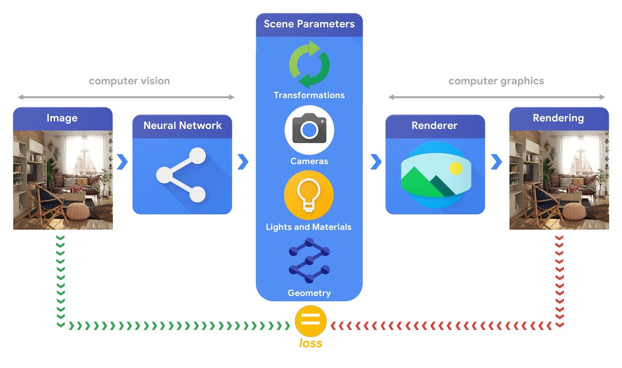
One solution for this problem is an unsupervised learning technique called “analysis by synthesis.” In this technique, similar to an autoencoder, the goal is for the neural network to simultaneously learn an encoder that converts an input into an intermediate representation, and a decoder that converts that intermediate representation into an output that, ideally, is exactly the same as the input. Of course it won’t be exact until the model is trained, and the difference between input and output, or loss, is used by the training algorithm called backpropagation to adjust the network parameters. Once the whole system is trained, the encoder can be used by itself as a computer vision system.
If the encoder learns a representation of an image that consists of a set of objects and their 3D-locations and orientations, then there are many 3D-graphics libraries such as OpenGL that can render this representation back into a high-quality image. Chaining the computer-vision encoder with the 3D-graphics rendering decoder provides an opportunity for unsupervised learning for computer vision using unlabelled datasets.
Source: https://github.com/tensorflow/graphics
The problem is that it is not possible to simply drop in just any 3D-graphics library. The key to training a neural network is backpropagation, and this requires that every layer in the network support automatic differentiation.
The good news is that 3D-graphics rendering is based on the same linear algebra operations that TensorFlow was written to optimize—this is, after all, the very reason that deep learning gets such a boost from graphics processing units or GPUs, the specialized hardware created to accelerate 3D-graphics rendering. The TensorFlow Graphics library provides several rendering functions implemented using TensorFlow linear algebra code, making them differentiable “for free.” These functions include:
- Transformations that define rotation and translation of objects from their original 3D-position
- Material models that define how light interacts with objects to change their appearance
- Camera models that define projections of objects onto the image plane
Besides the graphics rendering functions for the decoder, the library also includes new tools for the encoder section. Not all recognition tasks operate on rectangular grids of images; many 3D-sensors such as LIDARs provide data as a “point cloud” or mesh of connected points. This is challenging for common computer-vision neural network architectures such as convolutional neural networks (CNNs), which expect input data to be a map of a rectangular grid of points. TensorFlow Graphics provides new convolutional layers for mesh inputs. To assist developers in debugging their models, there is also a new TensorBoard plugin for visualizing point clouds and meshes.
Commenters on Hacker News reacted positively:
Nice! I played with OpenDR (http://files.is.tue.mpg.de/black/papers/OpenDR.pdf) a few years ago, and got really excited about it. Unfortunately it uses a custom autodiff implementation that made it hard it to integrate with other deep learning libraries. Pytorch still seems to be lagging in this area, bit there’s some interesting repos on github (e.g. https://github.com/daniilidis-group/neural_renderer).
Dimitri Diakopoulos, a researcher at Oculus, said on Twitter:
This codebase is a perfect compliment [sic] to Tzu-Mao Li’s recently published PhD thesis on Differentiable Visual Computing. His work brings the reader through the foundations of differentiable rendering theory through recent state-of-the-art. https://arxiv.org/abs/1904.12228
TensorFlow Graphics is available on GitHub.
MMS • RSS
Article originally posted on Data Science Central. Visit Data Science Central

The benefits of AI for healthcare have been extensively discussed in the recent years up to the point of the possibility to replace human physicians with AI in the future.
Both such discussions and the current AI-driven projects reveal that Artificial Intelligence can be used in healthcare in several ways:
- AI can learn features from a large volume of healthcare data, and then use the obtained insights to assist clinical practice in treatment design or risk assessment;
- AI system can extract useful information from a large patient population to assist making real-time inferences for health risk alert and health outcome prediction;
- AI can do repetitive jobs, such as analyzing tests, X-Rays, CT scans or data entry;
- AI systems can help to reduce diagnostic and therapeutic errors that are inevitable in the human clinical practice;
- AI can assist physicians by providing up-to-date medical information from journals, textbooks and clinical practices to inform proper patient care;
- AI can manage medical records and analyze both performance of an individual institution and the whole healthcare system;
- AI can help develop precision medicine and new drugs based on the faster processing of mutations and links to disease;
- AI can provide digital consultations and health monitoring services — to the extent of being “digital nurses” or “health bots”.
Despite the variety of applications of AI in the clinical studies and healthcare services, they fall into two major categories: analysis of structured data, including images, genes and biomarkers, and analysis of unstructured data, such as notes, medical journals or patients’ surveys to complement the structured data. The former approach is fueled by Machine Learning and Deep Learning Algorithms, while the latter rest on the specialized Natural Language Processing practices.
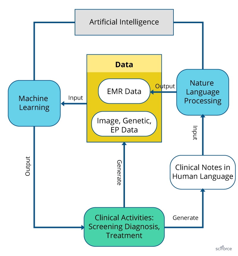
Figure 1. Machine Learning and Natural Language Processing in healthcare.
Machine Learning Algorithms
ML algorithms chiefly extract features from data, such as patients’ “traits” and medical outcomes of interest.
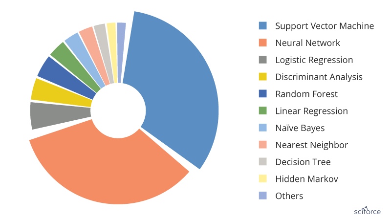
Figure 2. The most popular Machine Learning algorithms used in the medical literature. The data are generated through searching the Machine Learning algorithms within healthcare on PubMed
For a long time, AI in healthcare was dominated by the logistic regression, the most simple and common algorithm when it is necessary to classify things. It was easy to use, quick to finish and easy to interpret. However, in the past years the situation has changed and SVM and neural networks have taken the lead.
Support Vector Machine
Support Vector Machines (SVM) can be employed for classification and regression, but this algorithm is chiefly used in classification problems that require division of a dataset into two classes by a hyperplane. The goal is to choose a hyperplane with the greatest possible margin , or distance between the hyperplane and any point within the training set, so that new data can be classified correctly. Support vectors are data points that are closest to the hyperplane and that, if removed, would alter its position. In SVM, the determination of the model parameters is a convex optimization problem so the solution is always global optimum.
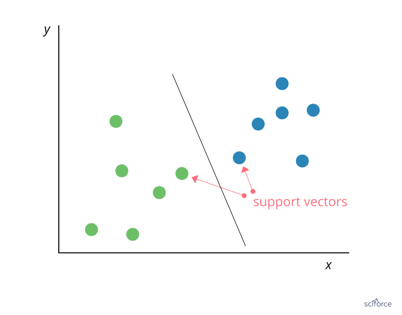
Figure 3. Support Vector Machine
SVMs are used extensively in clinical research, for example, to identify imaging biomarkers, to diagnose cancer or neurological diseases and in general for classification of data from imbalanced datasets or datasets with missing values.
Neural networks
In neural networks, the associations between the outcome and the input variables are depicted through hidden layer combinations of prespecified functionals. The goal is to estimate the weights through input and outcome data in such a way that the average error between the outcome and their predictions is minimized.
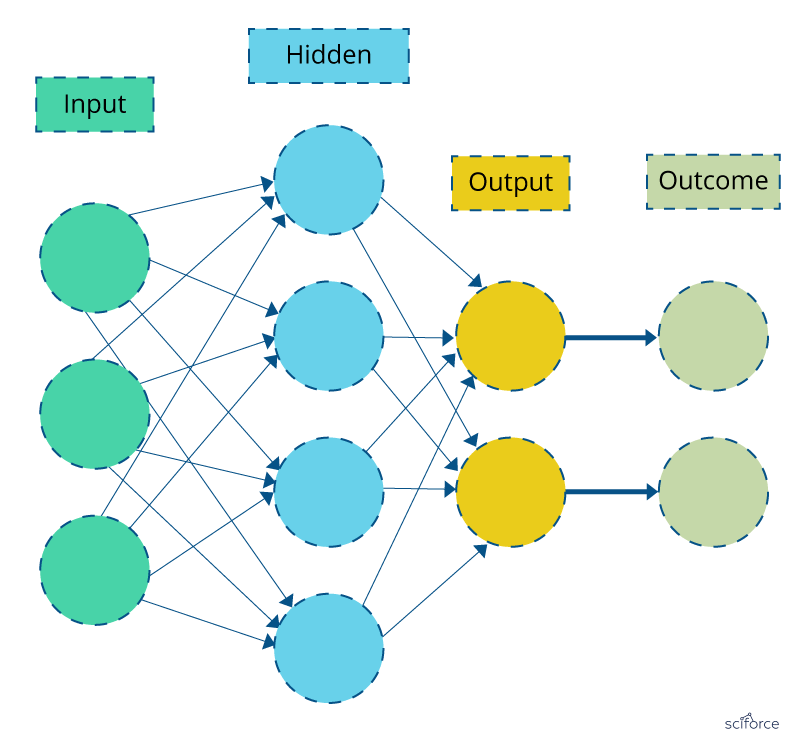
Figure 4. Neural Network
Neural networks are successfully applied to various areas of medicine, such as diagnostic systems, biochemical analysis, image analysis, and drug development, with the textbook example of breast cancer prediction from mammographic images.
Logistic Regression
Logistic Regression is one of the basic and still popular multivariable algorithms for modeling dichotomous outcomes. Logistic regression is used to obtain odds ratio when more than one explanatory variable is present. The procedure is similar to multiple linear regression, with the exception that the response variable is binomial. It shows the impact of each variable on the odds ratio of the observed event of interest. In contrast to linear regression, it avoids confounding effects by analyzing the association of all variables together.
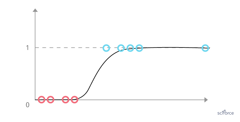
Figure 5. Logistic Regression
In healthcare, logistic regression is widely used to solve classification problems and to predict the probability of a certain event, which makes it a valuable tool for a disease risk assessment and improving medical decisions.
Natural Language Processing
In healthcare, a large proportion of clinical information is in the form of narrative text, such as physical examination, clinical laboratory reports, operative notes and discharge summaries, which are unstructured and incomprehensible for the computer program without special methods of text processing. Natural Language Processing addresses these issues as it identifies a series of disease-relevant keywords in the clinical notes based on the historical databases that after validation enter and enrich the structured data to support clinical decision making.
TF-IDF
Basic algorithm for extracting keywords, TF-IDF stands for term frequency-inverse document frequency. The TF-IDF weight is a statistical measure of a word importance to a document in a collection or corpus. The importance increases proportionally to the number of times a word appears in the document but is offset by the frequency of the word in the corpus.
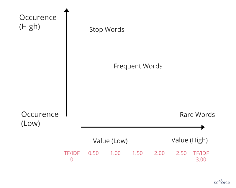
Figure 6. TF-IDF
In healthcare, TF-IDF is used in finding patients’ similarity in observational studies, as well as in discovering disease correlations from medical reports and finding sequential patterns in databases.
Naïve Bayes
Naïve Bayes classifier is a baseline method for text categorization, the problem of judging documents as belonging to one category or the other. Naive Bayes classifier assumes that the presence of a particular feature in a class is unrelated to the presence of any other feature. Even if these features are interdependent, all of these properties independently contribute to the probability of belonging to a certain category.
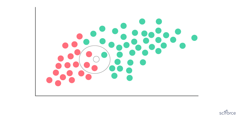
Figure 7. Naïve Bayes classifier
It remains one of the most effective and efficient classification algorithms and has been successfully applied to many medical problems, such as classification of medical reports and journal articles.
Word Vectors
Considered to be a breakthrough in NLP, word vectors, or word2vec, is a group of related models that are used to produce word embeddings. In their essence, word2vec models are shallow, two-layer neural networks that reconstruct linguistic contexts of words. Word2vec produces a multidimensional vector space out of a text, with each unique word having a corresponding vector. Word vectors are positioned in the vector space in a way that words that share contexts are located in close proximity to one another.
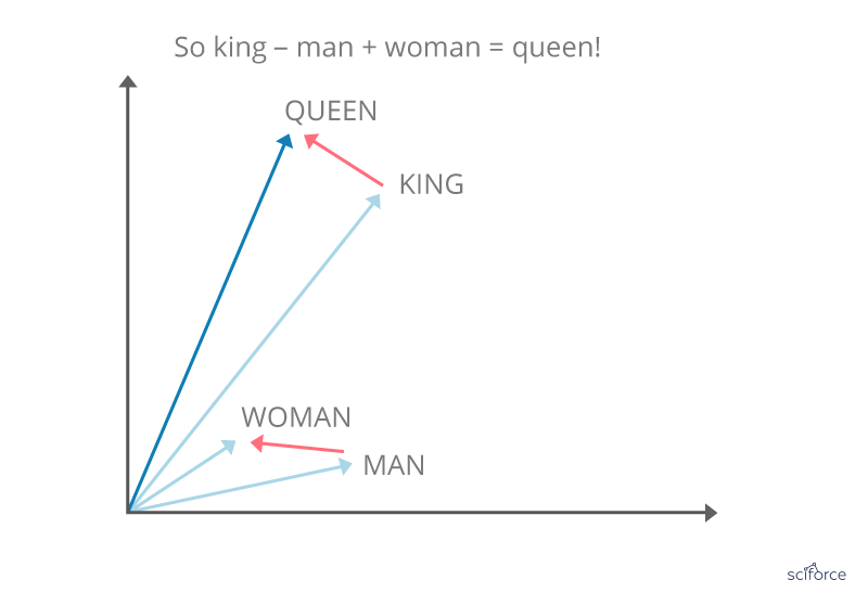
Figure 8. Word vectors
Word vectors are used for biomedical language processing, including similarity finding, medical terms standardization and discovering new aspects of diseases.
Deep Learning
Deep Learning is an extension of the classical neural network technique, being, to put it simply, as a neural network with many layers. Having more capacities compared to classical ML algorithms, Deep Learning can explore more complex non-linear patterns in the data. Being a pipeline of modules each of them are trainable, Deep Learning represents a scalable approach that, among others, can perform automatic feature extraction from raw data.
In the medical applications, Deep Learning algorithms successfully address both Machine Learning and Natural Language Processing tasks. The commonly used Deep Learning algorithms include convolution neural network (CNN), recurrent neural network, deep belief network and multilayer perception, with CNNs leading the race from 2016 on.
Convolutional Neural Network
The CNN was developed to handle high-dimensional data, or data with a large number of traits, such as images. Initially, as proposed by LeCun, the inputs for CNN were normalized pixel values on the images. Convolutional networks were inspired by biological processes in that the connectivity pattern between neurons resembles the organization of the animal visual cortex, with individual cortical neurons responding to stimuli only in a restricted region of the receptive field. However, the receptive fields of different neurons partially overlap such that they cover the entire visual field. The CNN then transfers the pixel values in the image by weighting in the convolution layers and sampling in the subsampling layers alternatively. The final output is a recursive function of the weighted input values.
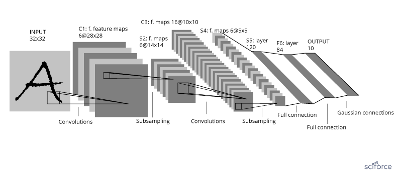
Figure 9. A convolutional neural network
Recently, the CNN has been successfully implemented in the medical area to assist disease diagnosis, such as skin cancer or cataracts.
Recurrent Neural Network
The second in popularity in healthcare, RNNs represent neural networks that make use of sequential information. RNNs are called recurrent because they perform the same task for every element of a sequence, and the output depends on the previous computations. RNNs have a “memory” which captures information about what has been calculated several steps back (more on this later).
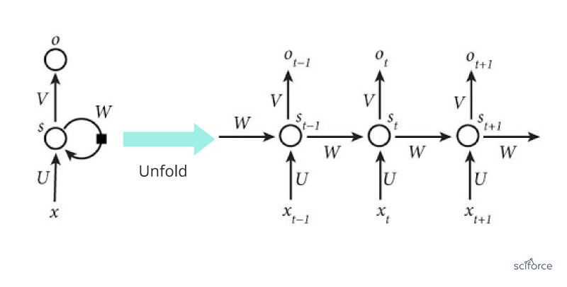
Figure 10. A recurrent neural network
Extremely popular in NLP, RNNs are also a powerful method of predicting clinical events.
Until recently, the AI applications in healthcare chiefly addressed a few disease types: cancer, nervous system disease and cardiovascular disease being the biggest ones. At present, advances in AI and NLP, and especially the development of Deep Learning algorithms have turned the healthcare industry to using AI methods in multiple spheres, from dataflow management to drug discovery.
MMS • RSS
Article originally posted on Data Science Central. Visit Data Science Central
This simple introduction to matrix theory offers a refreshing perspective on the subject. Using a basic concept that leads to a simple formula for the power of a matrix, we see how it can solve time series, Markov chains, linear regression, data reduction, principal components analysis (PCA) and other machine learning problems. These problems are usually solved with more advanced matrix calculus, including eigenvalues, diagonalization, generalized inverse matrices, and other types of matrix normalization. Our approach is more intuitive and thus appealing to professionals who do not have a strong mathematical background, or who have forgotten what they learned in math textbooks. It will also appeal to physicists and engineers. Finally, it leads to simple algorithms, for instance for matrix inversion. The classical statistician or data scientist will find our approach somewhat intriguing.
1. Power of a Matrix
For simplicity, we illustrate the methodology for a 2 x 2 matrix denoted as A. The generalization is straightforward. We provide a simple formula for the n-th power of A, where n is a positive integer. We then extend the formula to n = -1 (the most useful case) and to non-integer values of n.
Using the notation
we obtain
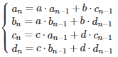
Using elementary substitutions, this leads to the following system:
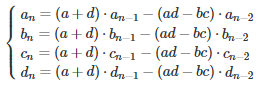
We are dealing with identical linear homogeneous recurrence relations. Only the initial conditions corresponding to n = 0 and n = 1, are different for these four equations. The solution to such equations is obtained as follows (see here for details.) First, solve the quadratic equation
The two solutions r(1), r(2) are
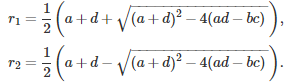
If the quantity under the square root is negative, then the roots are complex numbers. The final solution depends on whether the roots are distinct or not:
with
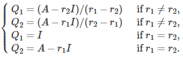
Here the symbol I represents the 2 x 2 identity matrix. The last four relationships were obtained by applying the above formula for A^n, with n = 0 and n = 1. It is easy to prove (by recursion on n) that this is the correct solution.
If none of the roots is zero, then the formula is still valid for n = -1, and thus it can be used to compute the inverse of A.
2. Examples, Generalization, and Matrix Inversion
For a p x p matrix, the methodology generalizes as follows. The quadratic polynomial becomes a polynomial of degree p, known as the characteristic polynomial. If its roots are distinct, we have
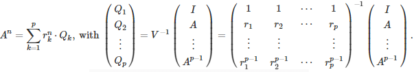
The matrix V is a Vandermonde matrix, so there is an explicit formula to compute its inverse, see here and here. A fast algorithm for the computation of its inverse is available here. The determinants of A and V are respectively equal to
Note that the roots can be real or complex numbers, simple or multiple, or equal to zero. Usually the roots are ordered by decreasing modulus, that is
That way, a good approximation for A^n is obtained by using the first three or four roots if n > 0, and the last three or four roots if n < 0. In the context of linear regression (where the core of the problem consists of inverting a matrix, that is, using n = -1 in our general formula) this approximation is equivalent to performing a principal component analysis (PCA) as well as PCA-induced data reduction.
If some roots have a multiplicity higher than one, the formulas must be adjusted. The solution can be found by looking at how to solve an homogeneous linear recurrence equation, see theorem 4 in this document.
2.1. Example with a non-invertible matrix
Even if A is non-invertible, some useful quantities can still be computed when n = -1, not unlike using a pseudo-inverse matrix in the general linear model in regression analysis. Let’s look at this example, using our own methodology:
The rightmost matrix attached to the second root 0 is of particular interest, and plays the role of a pseudo-inverse matrix for A. If that second root was very close to zero rather than exactly zero, then the term involving the rightmost matrix would largely dominate in the value of A^n, when n = -1. At the limit, some ratios involving the (non-existent!) inverse of A still make sense. For instance:
- The sum of the elements of the inverse of A, divided by its trace, is (4 – 2 – 2 + 1) / (4 + 1) = 1 / 5.
- The arithmetic mean divided by the geometric mean of its elements, is 1 / 2.
2.2. Fast computations
If n is large, one way to efficiently compute A^n is as follows. Let’s say that n = 100. Do the following computations:
This can be useful to quickly get an approximation of the largest root of the characteristic polynomial, by eliminating all but the first root in the formula for A^n, and using n = 100. Once the first root has been found, it is easy to also get an approximation for the second one, and then for the third one.
If instead, you are interested in approximating the smallest roots, you can proceed the other way around, by using the formula for A^n, with n = -100 this time.
3. Application to Machine Learning Problems
We have discussed principal component analysis, data reduction, and pseudo-inverse matrices in section 2. Here we focus on applications to time series, Markov chains, and linear regression.
3.1. Markov chains
A Markov chain is a particular type of time series or stochastic process. At iteration or time n, a system is in a particular state s with probability P(s | n). The probability to move from state s at time n, to state t at time n + 1 is called a transition probability, and does not depend on n, but only on s and t. The Markov chain is governed by its initial conditions (at n = 0) and the transition probability matrix denoted as A. The size of the transition matrix is p x p, where p is the number of potential states that the system can evolve to. As n tends to infinity A^n and the whole system reaches an equilibrium distribution. This is because
- The characteristic polynomial attached to A has a root equal to 1.
- The absolute value of any root is less than or equal to 1.
3.2. AR processes
Auto-regressive (AR) processes represent another basic type of time series. Unlike Markov chains, the number of potential states is infinite and forms a continuum. Yet the time is still discrete. Time-continuous AR processes such as Gaussian processes, are not included in this discussion. An AR(p) process is defined as follows:
Its characteristic polynomial is
Here { e(n) } is a white noise process (typically uncorrelated Gaussian variables with same variance) and we can assume that all expectations are zero. We are dealing here with a non-homogeneous linear (stochastic) recurrence relation. The most interesting case is when all the roots of the characteristic polynomial have absolute value less than 1. Processes satisfying this condition are called stationary. In that case, the auto-correlations are decaying exponentially fast.
The lag-k covariances satisfy the relation
with
Thus the auto-correlations can be explicitly computed, and are also related to the characteristic polynomial. This fact can be used for model fitting, as the auto-correlation structure uniquely characterizes the (stationary) time series. Note that if the white noise is Gaussian, then the X(n)’s are also Gaussian. The results about the auto-correlation structure can be found in this document, pages 98 and 106, originally posted here. See also this this document (pages 112 and 113) originally posted here, or the whole book (especially chapter 6) available here.
3.3. Linear regression
Linear regression problems can be solved using the OLS (ordinary least squares) method, see here. The framework involves a response y, a data set X consisting of p features or variables and m observations, and p regression coefficients (to be determined) stored in a vector b. In matrix notation, the problem consists of finding b that minimizes the distance ||y – Xb|| between y and Xb. The solution is
The techniques discussed in this article can be used to compute the inverse of A, either exactly using all the roots of its characteristic polynomial, or approximately using the last few roots with the lowest moduli, as if performing a principal component analysis. If A is not invertible, the methodology described in section 2.1. can be useful: it amounts to working with a pseudo inverse of A. Note that A is a p x p matrix as in section 2.
Questions regarding confidence intervals (for instance, for the coefficients) can be addressed using the model-free re-sampling techniques discussed in my article confidence intervals without pain.
To not miss this type of content in the future, subscribe to our newsletter. For related articles from the same author, click here or visit www.VincentGranville.com. Follow me on on LinkedIn, or visit my old web page here.
MMS • RSS
Article originally posted on InfoQ. Visit InfoQ
Capacitor, Ionic’s new native API container aimed to create iOS, Android, and Web apps using JavaScript, hit version 1.0. It attempts to bring a new take on how to build cross-platform apps that access native features.
Similarly to Cordova, Capacitor’s goal is to make possible to access native features of the OS underlying an app without requiring to write platform-specific code. This makes possible to use, for example, the device camera using the same code in iOS, Android, and Electron apps. Capacitor, though, takes a radically different approach to containerize an HTML/CSS/JavaScript app to run it into a native Web View and expose native functionality your app can use through a unified interface.
One major difference with Cordova is Capacitor requires developers to handle their native app project, the one that includes the Web View where the Ionic app is run, as a component of the Capacitor app rather than the opposite. This approach makes it easier to integrate external SDKs that may require tweaking the AppDelegate on iOS, as well as to integrate native functionality to the Ionic app without writing a proper plugin, as it was the case with Cordova.
Another benefit of Capacitor is it does not require you to listen to the deviceready event anymore. This is made possible by Capacitor loading all plugins before the Ionic app is loaded, so they are immediately available. Additionally, Capacitor plugins expose callable methods, so you do not need to use exec. For example, this is a very simple Capacitor plugin for iOS, a Swift class extending CAPPlugin:
import Capacitor

@objc(MyPlugin)
public class MyPlugin: CAPPlugin {
  @objc func echo(_ call: CAPPluginCall) {
    let value = call.getString("value") ?? ""
    call.resolve([
        "value": value
    ])
  }
}
To make the plugin echo method directly available to the Capacitor web runtime, you need to register it in a .m file:
#import <Capacitor/Capacitor.h>

CAP_PLUGIN(MyPlugin, "MyPlugin",
  CAP_PLUGIN_METHOD(echo, CAPPluginReturnPromise);
)
Capacitor uses npm for its dependency management, including plugins and platforms. So, when you need to use a plugin, you just run npm install as usual for JavaScript project. With Cordova, instead, you are required to use the cordova plugin add ... command. As an added simplification, Capacitor requires the native component of iOS plugins to be packaged as a CocoaPod, and for Android as a standalone library.
As a final note, Capacitor will eventually replace Cordova as the official way to containerize Ionic apps so they can access native features cross-platform, but Cordova will be supported for many years to come, Ionic says.
Real Time Computer Vision is Likely to be the Next Killer App but We’re Going to Need New Chips
MMS • RSS
Article originally posted on Data Science Central. Visit Data Science Central
Summary: Real Time Computer Vision (RTCV) that requires processing video DNNs at the edge is likely to be the next killer app that powers a renewed love affair with our mobile devices. The problem is that current GPUs won’t cut it and we have to wait once again for the hardware to catch up.

The entire history of machine learning and artificial intelligence (AI/ML) has been a story about the race between techniques and hardware. There have been times when we had the techniques but the hardware couldn’t keep up. Conversely there have been times when hardware has outstripped technique. Candidly though, it’s been mostly about waiting for the hardware to catch up.
You may not have thought about it, but we’re in one of those wait-for-tech hardware valleys right now. Sure there’s lots of cloud based compute and ever faster GPU chips to make CNN and RNN work. But the barrier that we’re up against is latency, particularly in computer vision.
If you want to utilize computer vision on your cell phone or any other edge device (did you ever think of self-driving cars as edge devices) then the data has to make the full round trip from your local camera to the cloud compute and back again before anything can happen.
There are some nifty applications that are just fine with delays of say 200 ms or even longer. Most healthcare applications are fine with that as are chatbots and text/voice apps. Certainly search and ecommerce don’t mind.
But the fact is that those apps are rapidly approaching saturation. Maturity if you’d like a kinder word. They don’t thrill us any longer. Been there, done that. Competing apps are working for incremental share of attention and the economics are starting to work against them. If you’re innovating with this round-trip data model, you’re probably too late.
What everyone really wants to know is what’s the next big thing. What will cause us to become even more attached to our cell phones, or perhaps our smart earbuds or augmented glasses. That thing is most likely to be ‘edge’ or ‘real time computer vision’ (RTCV).
What Can RTCV Do that Regular Computer Vision Can’t
Pretty much any task that relies on movie-like live vision (30 fps, roughly 33 ms response or better) can’t really be addressed by the round-trip data model. Here are just a few: drones, autonomous vehicles, augmented reality, robotics, cashierless checkout, video monitoring for retail theft, monitoring for driver alertness.
Wait a minute you say. All those things currently exist and function. Well yes and no. Everyone’s working on chips to make this faster but there’s a cliff coming in two forms. First, the sort of Moore’s law that applies to this round-trip speed, and second the sheer volume of devices that want to utilize RTCV.
What about 5G? That’s a temporary plug. The fact is that the round-trip data architecture is at some level always going to be inefficient and what we need is a chip that can do RTCV that is sufficiently small enough, cheap enough, and fast enough to live directly on our phone or other edge device.
By the way, if the processing is happening on your phone then the potential for hacking the data stream goes completely away.
AR Enhanced Navigation is Most Likely to be the Killer App
Here’s a screen shot of an app called Phiar, shown by co-founder and CEO Chen Ping Yu at last week’s ‘Inside AI Live’ event.

Chen Ping’s point is simple. Since the camera on our phone is most likely already facing forward, why not just overlay the instruction directly on the image AR-style and eliminate the confusion caused by having to glance elsewhere at a more confusing 2D map.
This type of app requires that minimum 30 FPS processing speed (or faster). Essentially AR overlays on real time images is the core of RTCV and you can begin to see the attraction.
The Needed Compute is Just Going Wild
Even without RTCV, our most successful DNNs are winning by using increasingly larger amounts of compute.
Gordon Wilson, CEO of RAIN Neuromorphics used this graph at that same ‘Inside AI Live’ event to illustrate these points. Since our success with AlexNet in 2012 to AlphaGo in 2018, the breakthrough winners have done it with a 300,000x increase in needed compute.
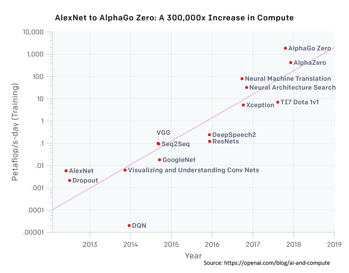
That doubling every 3 ½ months is driven by ever larger DNNs with more neurons processing more features and ever larger datasets. And to be specific, it’s not that our DNNs are just getting deeper with more layers, the real problem is that they need to get wider, with more input neurons corresponding to more features.
What’s Wrong with Simply More and Faster GPUs?
Despite the best efforts of Nvidia, the clear king of GPUs for DNN, the hardware stack needed to train and run computer vision apps is about the size of three or four laptops stacked on top of each other. That’s not going to fit in your phone.
For some really interesting technical reasons that we’ll discuss in our next article, it’s not likely that GPUs are going to cut it for next gen edge processing of computer vision in real time.
The good news is that there are on the order of 100 companies working on AI-specific silicon, ranging from the giants like Nvidia down to a host of startups. Perhaps most interesting is that this app will introduce the era of the neuromorphic chip. More on the details next week.
Other articles by Bill Vorhies
About the author: Bill is Contributing Editor for Data Science Central. Bill is also President & Chief Data Scientist at Data-Magnum and has practiced as a data scientist since 2001. His articles have been read more than 1.5 million times.
He can be reached at:
Podcast: Nick White on the Lessons Software Engineering Can Learn from Multi-disciplinary Medical Teams
MMS • RSS
Article originally posted on InfoQ. Visit InfoQ
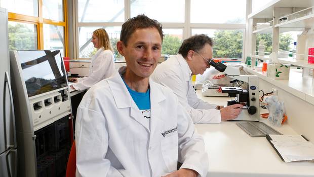
In this podcast, Shane Hastie, Lead Editor for Culture & Methods, spoke to Nick White about his experiences as a medical patient under the care of a cross-functional, multi-disciplinary team and the lessons that we can take from that for software engineering.
Key Takeaways
- The collaborative approach to diagnosis by a multi-disciplinary team of specialists used by the Wellington Regional Hospital Cancer Care Unit
- With a complex diagnosis like cancer, the range of treatment options is wide and the multi-disciplinary approach enables the best possible combination of treatments and more successful patient outcomes
- Setting a goal of coming back from the surgery to continue as a mountain runner
- Running up Mt Fuji to raise funds and awareness for cancer research
- As technologists we need to be open to learning from other disciplines in areas such as collaboration approaches, dealing with hand-offs and bottle-necks, and customer service
Subscribe on:
Show Notes
- 00:45 Introductions
- 01:09 The high-stakes environment of medical care
- 02:02 Nick’s story of being diagnosed with cancer
- 04:23 The shock of the diagnosis and the impact on Nick, his family and friends
- 05:23 The multi-disciplined approach taken by the cancer treatment unit in Wellington Regional Hospital
- 06:10 The contrast between this approach and the normal experience of dealing with medical specialists on at a time
- 06:24 Why this approach is preferred for cancer treatment
- 07:24 Coming to a consensus opinion quickly and identifying treatment options
- 08:14 Describing the extensive surgery and treatment Nick was to go through
- 10:54 24 hours to tell friends and family that he was going in for radical and high-risk surgery
- 12:35 Coming through the surgery and being unable to speak – communicating using hand-written notes
- 13:14 The process of getting speech back over 6 months
- 14:16 Setting goals to come back from the illness to do mountain running
- 15:18 Registering the run The Goat mountain race prior to the surgery (6 months after the surgery)
- 16:42 The physical recovery process
- 17:47 Sneaking in activities to prepare for mountain running
- 19:00 Running The Goat six months after surgery
- 19:35 Continuing mountain running as the recovery progressed
- 20:54 The path to recovery was not straightforward, there were setbacks and problems along the way
- 22:16 The value of positive stories for people who are going through cancer treatment
- 22:47 5 years after surgery patients are considered cancer-free and Nick wanted to do something meaningful to mark the milestone
- 22:57 Deciding to run up Mt Fuji in Japan to raise funds and awareness for cancer research
- 23:54 The challenges involved with tackling Mt Fuji
- 24:48 The goal of running up Mt Fuji and returning to Wellington to give a speech about it to raise funds for the Gillies McIndoe Research Institute
- 26:17 The goal was to raise $3776, the actual figure raised was $8000
- 26:48 Bringing these experiences and ideas into working with technical teams as an agile coach
- 27:03 The importance of trust and communication when under pressure and the stakes are high
- 27:57 How multi-disciplinary medical teams tackle the problem of hand-offs can provide guidance for software teams
- 29:09 Be open to learning from other disciplines and approaches
- 29:57 The example of adventure racing – what ideas can technical teams learn from the way those teams support each other?
- 30:39 The best teams have a mix of different skills
- 31:30 Advice for the audience: Look beyond your own profession, see what you can learn from different professions, industries and disciplines and bring the ideas into your own work
Mentioned:
From time to time InfoQ publishes trend reports on the key topics we’re following, including a recent one on DevOps and Cloud. So if you are curious about how we see that state of adoption for topics like Kubernetes, Chaos Engineering, or AIOps point a browser to http://infoq.link/devops-trends-2019.
More about our podcasts
You can keep up-to-date with the podcasts via our RSS Feed, and they are available via SoundCloud, Apple Podcasts, Spotify, Overcast and the Google Podcast. From this page you also have access to our recorded show notes. They all have clickable links that will take you directly to that part of the audio.
Previous podcasts
MMS • RSS
Article originally posted on Data Science Central. Visit Data Science Central
A.I. based automated Anomaly detection system is gaining popularity nowadays due to the increase in data generated from various devices and the increase in ever evolving sophisticated threats from hackers etc. Anomaly detection systems can be applied across various business scenarios like monitoring financial transactions of a fintech company, highlighting fraudulent activities in a network, e-commerce price glitches among millions of products, and so on. Anomaly detection system can work well in managing millions of metrics at scale and filter them into a number of consumable incidents to create actionable insights.
While deploying the right anomaly detection system, companies should ask the following important questions to ensure the deployment of the correct product for their needs:
1] What is the alert frequency (5 minutes/ 10 minutes/ 1 hour or 1 day)
2] Requirement of a scalable solution (Big data vs. regular RDBMS data)
3] On-premise or cloud-based solution (Docker vs. AWS EC instance)
4] Unsupervised vs. Semi-supervised solution
5] How to read & prioritize various anomalies in order to take appropriate action (Point based vs. Contextual vs. Collective anomalies)
6] Alert integration with systems
What is the alert frequency (5 minutes/ 10 minutes/ 1 hour or 1 day): Alert frequency is very much dependent on the sensitivity of the process which will be being measured, including the reaction time and other metrics. Some applications demand low latency: like detecting & intimating the suspicious fraudulent payment transactions to users in case of any misuse of the card within minutes. In the case of some applications it can be less sensitive to changes and not so severe, like total inbound & outbound calls from cellular towers, which can be aggregated to an hourly level rather than measuring at 5-minute intervals etc. One can choose between too much sensitivity and right number of alerts while measuring processes as per the suitability etc.
Requirement of the scalable solution (Big data vs. regular RDBMS data): Some businesses like e-commerce or fintech, need to save their data in a Big data environment due to its velocity or scalability. Whereas in other areas like banking, they can take comfort of using mainframe systems. In big data scenarios, hardware and software scalability needs to be taken care by systems like Hadoop and Spark respectively, vis-a-vis RDBMS and Python programming in regular scenarios.
On-premise or cloud-based solution (Docker vs. AWS EC instance): In the case of certain businesses such as fintech and banking, data cannot be dumped in the cloud, due to issues pertaining to compliance and confidentiality. For some other businesses like E-commerce, where said issues are not a factor, the data can be uploaded into a private cloud. Anomaly detection solutions should consider these aspects to understand if the deployment can happen either in Docker format for on-premise services or AWS based EC solution for cloud-based requirement.
Unsupervised vs. Semi-supervised solution: While deploying unsupervised learning algorithms to detect anomalies on time series-based data is a common solution, these systems are infamous for generating a high number of false positives. In this case, if businesses find there are high number of alerts, they can prioritize the alerts based on score and they can set higher threshold scores to increase focus towards critical anomalies. But, semi-supervised algorithms also do exist, which enable algorithms to re-train based on user feedback upon generated anomalies. This will enable algorithms to get trained to not repeat such mistakes at later stages. But it is important to bear in mind that integrating semi-supervised algorithms does come with its own challenges.
How to read & prioritize various anomalies in order to take action: Anomalies types vary in nature: point based, contextual & collective. Point based anomalies are anomalies generated from individual series which could be one-on-one in isolation. Contextual anomalies are the anomalies which appear as an anomaly at different time period, else it would be considered as normal data points. Example of contextual anomalies could be, if there is a surge in call volume during afternoon would not be considered as an anomaly, whereas if the same volume of surge happens during midnight, it would be considered as an anomaly. Contextual anomalies also appear on individual series, similar to point based anomaly. Finally, collective anomalies appear across various data series and these collections try to create a complete story. Companies should define the type of anomalies they are looking for in order to get the most out of the anomaly detection system. In addition, by prioritizing anomalies based on a scoring system, higher level anomalies can be given more preference.
Alert integration with systems: Once the alerts have been generated, it needs to be integrated with the available in-house systems. If this is not taken care of, resources will need to be employed for the verification process which can become tedious, especially in the case of false positives. Ideally alerts from anomaly detection systems should be integrated with email notification system, SMS notification system or any other dashboard system which can send notifications to users on the detection of glitches.
Conclusion: It has been evident that as a part of the evolution, explosion of data generated from various devices and applications in coming future. Technology is always been a double edge sword, with the great benefits it will also do come up with great challenges, including misuse, hacking, safety issues etc. By deploying the artificial intelligence enabled anomaly detection systems will be handy in combating these issues, by selecting appropriate configurations business can obtain best possible performances.
This article was originally published by CrunchMetrics
MMS • RSS
Article originally posted on Data Science Central. Visit Data Science Central
All the data we need today is already available on the internet, which is great news for data scientists. The only barrier to using this data is the ability to access it. There are some platforms that even include APIs (such as Twitter) that support data collection from web pages, but it is not possible to crawl most web pages using this advantage..
This article is written by Olgun Aydin, the author of the book R Web Scraping Quick Start Guide.
Before we go on to scrape the web with R, we need to specify that this is advanced data analysis, data collection. We will use the Hadley Wickham’s method for web scraping using rvest. The package also requires selectr and xml2 packages.
The way to operate the rvest pole is simple and straightforward. Just as we first made web pages manually, the rvest package defines the web page link as the first step. After that, appropriate labels have to be defined. The HTML language edits content using various tags and selectors. These selectors must be identified and marked for storage of their contents by the harvest package. Then, all the engraved data can be transformed into an appropriate dataset, and analysis can be performed.
rvest is a very useful R library that helps you collect information from web pages. It is designed to work with magrittr, inspired by libraries such as BeatifulSoup.
To start the web scraping process, you first need to master the R bases. In this section, we will perform web scraping step by step, using the rvest R package written by Hadley Wickham.
For more information about the rvesr package, visit the following URLs.
CRAN Page: https://cran.r-project.org/web/packages/rvest/index.html rvest on github: https://github.com/hadley/rvest.
After talking about the fundamentals of the rvest library, now we are going to deep dive into web scraping with rvest. We are going to talk about how to collect URLs from the website we would like to scrape.
We will use some simple regex rules for this issue. Once we have XPath rules and regex rules ready, we will jump into writing scripts to collect data from the website.
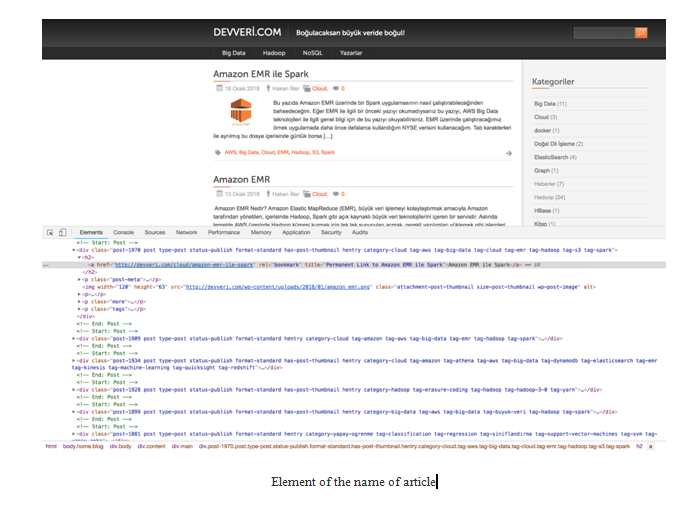
We will collect a dataset from a blog, which is about big data (www.devveri.com). This website provides useful information about big data, data science domains. It is totally free of charge. People can visit this website and find use cases, exercises, and discussions regarding big-data technologies.
Let’s start collecting information to find out how many articles there are in each category. You can find this information on the main page of the blog, using the following URL: http://devveri.com/ .
The screenshot shown is about the main page of the blog.
- As you see on the left-hand side, there are articles that were published recently. On the right-hand side, you can see categories and article counts of each categories:
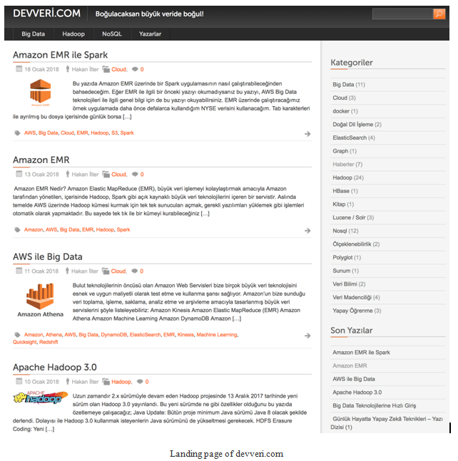
- To collect the information about how many articles we have for each categories, we will use the landing page URL of the website. We will be interested in the right-hand side of the web page shown in the following image:
- The following codes could be used to load the library and store the URL to the variable:
library(rvest)
urls<- “http://devveri.com/”
- If we print the URLs variable, it will look like the following image on the R Studio:
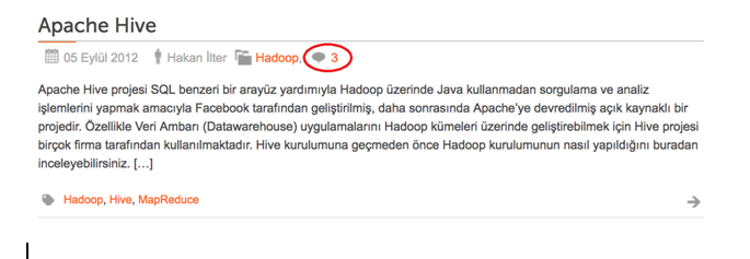
Now let’s talk about the comment counts of the articles. Because this web page is about sharing useful information about recent technologies regarding current development in the big-data and data science domain, readers can easily ask questions to the author or discuss about the article with other readers easily just by commenting to articles.
Also, it’s easy to see comment counts for each article on the category page. You can see one of the articles that was already commented on by readers in following screenshot. As you see, this article was commented on three times:
Now, we are going to create our XPath rules to parse the HTML document we will collect:
- First of all, we will write XPath rules to collect information from the left-hand side of the web page, in other words, to collect information about how many articles there are for each categories.
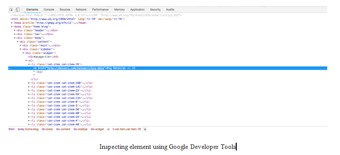
- Let’s navigate the landing page of the website com. As we exercised in previous chapter, will use Google Developer Tools to create and test XPath rules.
- To use Google Developer Tools, we can right-click on an element, which we are interested in extracting data from.
- Click Inspect Element.
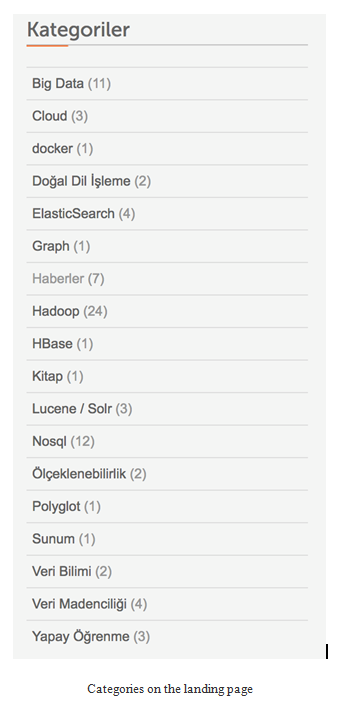
- On the following screenshot, we marked the elements regarding categories:
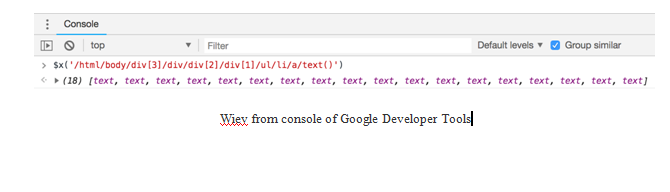
- Let’s write XPath rules to get the categories. We are looking for the information about how many article there are for each categories and the name of the categories:
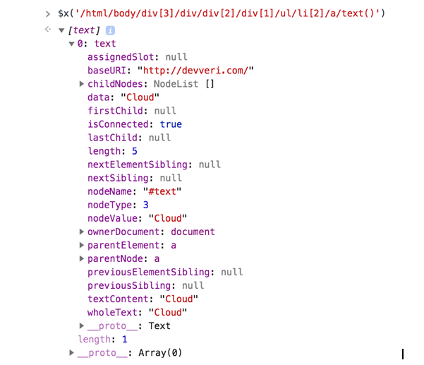
$x(‘/html/body/div[3]/div/div[2]/div[1]/ul/li/a/text()’)
- If you type the XPath rule to the console on the Developer Tools, you will get the following elements. As you can see, we have eighteen text elements, because there are eighteen categories shown on the right-hand side of the page:
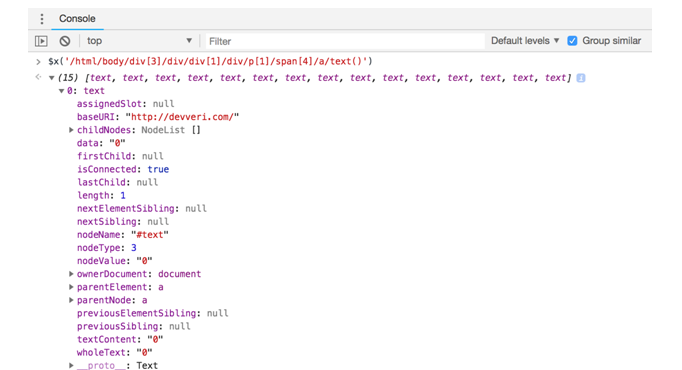
- Let’s open a text element and see how it looks. As you see, we managed to get the text content, which we are interested in.
In the next part, we will experience how to manage to extract this information with R. As you can see from the wholeText section, we only have category names:
Still, we will need to collect article counts for each categories:
- Use the following XPath rule; it will help to collect this information from the web page.
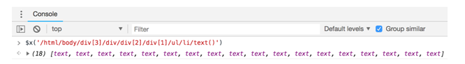
$x(‘/html/body/div[3]/div/div[2]/div[1]/ul/li/text()’)
- If you type the XPath rule to the console on the Developer Tools, you will get the following elements.
As you can see, we have 18 text elements, because there are eighteen categories shown on the right-hand side of the page:
Now it’s time to start collecting URLs for articles. Because, at this stage, we are going to collect comment counts for articles that were written recently. For this issue, it would be good to have the article name and the date of the articles. If we write the name of the first article, we will get the element regarding the name of the article, as shown in the following screenshot:
- Let’s write XPath rules to get the name of the article. We are looking for the name of the article:
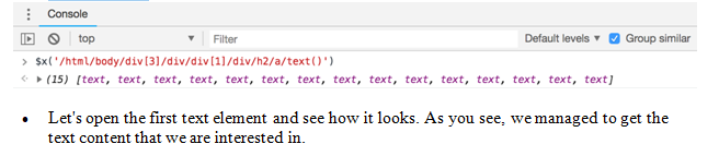
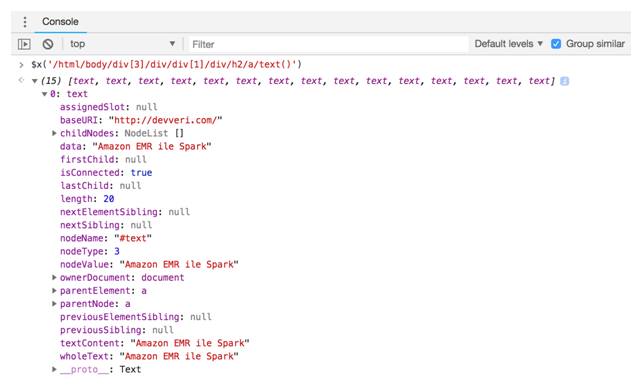
$x(‘/html/body/div[3]/div/div[1]/div/h2/a/text()’)
- If you type the XPath rule to the Developer Tools console, you will get the following elements. As you can see, we have 15 text elements, because there are 15 article previews on this page:
In the next part, we will experience how to extract this information with R:
We have the names of the articles, as we decided we should also collect the date and comment counts of the articles:
- The following XPath rule will help us to collect created date of the articles in text format:
$x(‘/html/body/div[3]/div/div[1]/div/p[1]/span[1]/text()’)
- If you type the XPath rule on the Developer Tools console, you will get the elements, as shown in the following screenshot:
As you can see, we have 15 text elements regarding dates, because there are 15 article previews on this page:
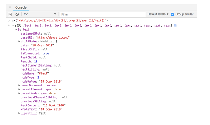
- Let’s open the first text element and see how it looks.
As you can see, we managed to get the text content that we are interested in. In the next part, we will experience how to extract this information with R:
We have the names of the articles and have created dates of the articles. As we decided, we should still collect the comment counts of the articles:
- The following XPath rule will help us to collect comment counts:
$x(‘/html/body/div[3]/div/div[1]/div/p[1]/span[4]/a/text()’)
- If you type the XPath rule to the Developer Tools console, you will get the elements, as shown in the following screenshot.
As you can see, we have 15 text elements regarding comment counts, because there are fifteen article previews on this page:
- Let’s open the first text element and see how it looks.
You see, we managed to get the text content that we are interested in. In the next part, we will experience how to extract this information with R:
Let’s start to write our first scraping using R. We have already created XPath rules and URLs that we are interested in. We will start by collecting category counts and information about how many articles there are for each category:
- First of all, we have called an rvest library using the library function. We should load the rvest library using the following command:
library(rvest)
- Now we need to create NULL variables, because we are going to save count of articles for each categories and the name of the categories.
- For this purpose, we are creating category and count variables:
#creating NULL variables
category<- NULL
count <- NULL
- Now it’s time to create a variable that includes the URL that we would like to navigate and collect data.
- As we mentioned in the previous section, we would like to collect data from first page of the website. By using the following code block, we are assigning a URL to the URLs variable:
#links for page
urls<- “http://devveri.com/”
Now for the most exciting part: Collecting data!
The following script is first of all visit the URL of the web page, collecting HTML nodes using the read_html function. To parse HTML nodes, we are using XPath rules that we have already created in the previous section. For this issue, we are using the html_nodes function, and we are defining our XPath rules ,which we already have, inside the function:
library(rvest)
#creating NULL variables
category<- NULL
count <- NULL
#links for page
urls<- “http://devveri.com/”
#reading main url
h <- read_html(urls)
#getting categories
c<- html_nodes(h, xpath = ‘/html/body/div[3]/div/div[2]/div[1]/ul/li/a/text()’)
#getting counts
cc<- html_nodes(h, xpath = ‘/html/body/div[3]/div/div[2]/div[1]/ul/li/text()’)
#saving results, converting XMLs to character
category<- as.matrix(as.character(c))
count<- as.matrix(as.character(cc))
- We can use the framefunction to see categories and counts together.
- You will get the following result on R, when you run the script on the first line as shown in the following code block:
>data.frame(category,count)
category count
1 Big Data (11)n
2 Cloud (3)n
3 docker (1)n
4 DoğalDilİşleme (2)n
5 ElasticSearch (4)n
6 Graph (1)n
7 Haberler (7)n
8 Hadoop (24)n
9 HBase (1)n
10 Kitap (1)n
11 Lucene / Solr (3)n
12 Nosql (12)n
13 Ölçeklenebilirlik (2)n
14 Polyglot (1)n
15 Sunum (1)n
16 VeriBilimi (2)n
17 VeriMadenciliği (4)n
18 YapayÖğrenme (3)n
MMS • RSS
Article originally posted on InfoQ. Visit InfoQ
About the conference

Code Mesh LDN, the Alternative Programming Conference, focuses on promoting useful non-mainstream technologies to the software industry. The underlying theme is “the right tool for the job”, as opposed to automatically choosing the tool at hand.