Article originally posted on Data Science Central. Visit Data Science Central

Azure Machine Learning concepts – an Introduction

Introduction

Last week, we launched a free book called Classification and Regression in a weekend. The idea of the ‘in a weekend’ series of books is to study one complex section of code in a weekend to master the concept. This week. we plan to launch a book called “An Introduction to Azure Machine Learning in a Weekend”. This blog relates to the forthcoming book. If you don’t have an Azure subscription, you can use the free or paid version of Azure Machine Learning service. It is important to delete resources after use.

Azure Machine Learning service is a cloud service that you use to train, deploy, automate, and manage machine learning models – availing all the benefits of a Cloud deployment.

In terms of development, you can use Jupyter notebooks and the Azure SDKs. You can see more details of the Azure Machine Learning Python SDK which allow you to choose environments like Scikit-learn, Tensorflow, PyTorch, and MXNet.

Sequence of flow

Source: https://docs.microsoft.com/en-gb/azure/machine-learning/service/overview-what-is-azure-ml

The Azure machine learning workflow generally follows this sequence:

1. Develop machine learning training scripts in Python.
2. Create and configure a compute target.
3. Submit the scripts to the configured compute target to run in that environment. During training, the scripts can read from or write to datastore. And the records of execution are saved as runs in the workspace and grouped under experiments.
4. Query the experiment for logged metrics from the current and past runs. If the metrics don’t indicate a desired outcome, loop back to step 1 and iterate on your scripts.
5. After a satisfactory run is found, register the persisted model in the model registry.
6. Develop a scoring script that uses the model and Deploy the model as a web service in Azure, or to an IoT Edge device.

Below, we explain some concepts relating to running machine learning algorithms in the Azure Cloud as per the above flow

The workspace is the top-level resource for Azure Machine Learning service. It provides a centralized place to work with all the artefacts you create when you use Azure Machine Learning service. The workspace keeps a history of all training runs, including logs, metrics, output, and a snapshot of your scripts.

Once you have a model you like, you register it with the workspace. You then use the registered model and scoring scripts to deploy to Azure Container Instances, Azure Kubernetes Service, or to a field-programmable gate array (FPGA) as a REST-based HTTP endpoint. You can also deploy the model to an Azure IoT Edge device as a module.

When you create a new workspace, it automatically creates several Azure resources that are used by the workspace:

• Azure Container Registry: Registers docker containers that you use during training and when you deploy a model.
• Azure Storage account: Is used as the default datastore for the workspace
• Azure Application Insights: Stores monitoring information about your models.
• Azure Key Vault: Stores secrets that are used by compute targets and other sensitive information that’s needed by the workspace.

An experiment is a grouping of many runs from a specified script. It is always associated to a workspace.

A model: has the same meaning as in traditional machine learning. In Azure, a model is produced by a run but models trained outside Azure can also be used.  Azure Machine Learning service is framework agnostic i.e.  popular machine learning frameworks such as Scikit-learn, XGBoost, PyTorch, TensorFlow etc can be used.

The model registry keeps track of all the models in your Azure Machine Learning service workspace.

A run configuration is a set of instructions that defines how a script should be run in a specified compute target. The configuration includes a wide set of behavior definitions, such as whether to use an existing Python environment or to use a Conda environment that’s built from a specification

Azure Machine Learning Datasets manage data in various scenarios such as model training and pipeline creation. Using the Azure Machine Learning SDK, you can access underlying storage, explore and prepare data, manage the life cycle of different Dataset definitions, and compare between Datasets used in training and in production.

A datastore is a storage abstraction over an Azure storage account. The datastore can use either an Azure blob container or an Azure file share as the back-end storage. Each workspace has a default datastore, and you can register additional datastores. You can use the Python SDK API or the Azure Machine Learning CLI to store and retrieve files from the datastore.

A compute target is the compute resource that you use to run your training script or host your service deployment. Your local computer, A linux VM in Azure; Azure Databricks etc are all examples of compute targets

A training script – brings it all together. During training, the directory containing the training script and the associated files is copied to the compute target and executed there. A snapshot of the directory is also stored under the experiment in the workspace.

A run – A run is produced when you submit a script to train a model. A run is a record that contains information like the metadata about the run, output files, metrics etc

Github tracking and integration – When you start a training run where the source directory is a local Git repository, information about the repository is stored in the run history.

Snapshot – snapshot(of a run) represents compressed directory that contains the script as a zip file maintained as a record. The snapshot is also sent to the compute target where the zip file is extracted and the script is run there.

An activity represents a long running operation. Creating or deleting a compute target. Running a script on the compute target etc are all examples of activities.

Image Images provide a way to reliably deploy a model, along with all components you need to use the model. An image contains of a model, scoring script or application and dependencies that are needed by the model/scoring script/application

Azure Machine Learning can create two types of images:

• FPGA image: Used when you deploy to a field-programmable gate array in Azure.
• Docker image: Used when you deploy to compute targets other than FPGA. Examples are Azure Container Instances and Azure Kubernetes Service.

Image registry: The image registry keeps track of images that are created from your models. You can provide additional metadata tags when you create the image.

Deployment

A deployment is an instantiation of your model into either a web service that can be hosted in the cloud or an IoT module for integrated device deployments.

Web service: A deployed web service can use Azure Container Instances, Azure Kubernetes Service, or FPGAs. You create the service from your model, script, and associated files. These are encapsulated in an image, which provides the run time environment for the web service. The image has a load-balanced, HTTP endpoint that receives scoring requests that are sent to the web service.

Iot module: A deployed IoT module is a Docker container that includes your model and associated script or application and any additional dependencies. You deploy these modules by using Azure IoT Edge on edge devices.

Pipelines: You use machine learning pipelines to create and manage workflows that stitch together machine learning phases. For example, a pipeline might include data preparation, model training, model deployment, and inference/scoring phases. Each phase can encompass multiple steps, each of which can run unattended in various compute targets.

Conclusion

We hope that this blog provides a simple framework to understand Azure. The blog is  based on the Azure documentation here.

Article originally posted on Data Science Central. Visit Data Science Central

Monday newsletter published by Data Science Central. Previous editions can be found here. The contribution flagged with a + is our selection for the picture of the week. To subscribe, follow this link.  

Announcements

• Chick-fil-A is seeking multiple experienced Data Scientists with expertise in either NLP, computer vision, or forecasting.  The right candidate will have demonstrated experience in both the theory and application of the relevant machine learning techniques.  In-depth experience with R or Python is a must, and experience with cloud deployment of ML/AI models is preferred. Click here to learn more and apply!
• Earn a big data degree with certs built in. You’re already a master of the dataset. Now take your existing credentials and turn them up a degree—earn your M.S. in Data Analytics online at WGU. Our IT programs are designed by industry experts, and because our curriculum is competency-based, you can move quickly through familiar concepts. Current SAS 9 certifications are included. Get more info here.

Featured Resources and Technical Contributions 

• Cross Validation in One Picture +
• Azure Machine Learning concepts – an Introduction
• Create Transformed Polygons Using the Covariance Matrix 
• Data Science Job in 90 days – Book Summary 
• Free Book: Foundations of Data Science (from Microsoft Research Lab) 
• Deep Learning Explainability: Hints from Physics 
• How to Install and Run Hadoop on Windows for Beginners 
• 29 Statistical Concepts Explained in Simple English – Part 13 
• A Complete Machine Learning Project Walk-Through in Python 
• Free Textbook: Probability Course, Harvard University (Based on R) 
• 19 Courses (MOOC) on Math & Stats for Data Science & Machine Learning 
• An Introduction to Python Virtual Environment 

Forum Questions

• Question: Recommendation system evaluation 
• Question: Record linkage (unsupervised learning) 
• Question: Statistical significance match with multi-variables 
• Question: Scanned documents OCR data cleaning 
• Question: Traffic/commute data and processing 
• Question: Moments of Order Statistics 
• Question about the big O notation 
• Question: Data science audio book for layperson 

Featured Articles and Forum Questions

• Xaas Business Model: Economics Meets Analytics 
• Should You Be Recommending Deep Learning Solutions in Your Company? 
• Profiling Store Visitors 
• Frame a problem as a machine learning problem or otherwise 
• What is Data Lake and How to Improve Data Lake Quality 
• Artificial Intelligence Continues Where Analytics Ends? 
• Implementing Knowledge Graphs in Enterprises – Some Tips and Trends 
• Price Forecasting: Electricity, Flights, Hotels, Real Estate, and Stock Pricing 
• Technology Use as a Function of Device Type 
• Unsupervised learning and its role in the knowledge discovery process 
• Prediction of Customer Churn with Machine Learning 

Picture of the Week

Source: article flagged with a + 

From our Sponsors

• NVIDIA – Delivering Faster Time to Insight
• Python & R Notebooks that level up your organization
• Treat yourself to the best data event of the year
• The Convergence of RPA and Automated Machine Learning
• Scale AI/ML with Data Wrangling Featuring Forrester – June 5
• Standardizing the Machine Learning Lifecycle – eBook
• Balancing AI Endeavors with Analytic Talent – DSC Podcast
• Free Book: Classification and Regression In a Weekend (members only)
• Free Book: Applied Stochastic Processes (members only)
• New Book: Enterprise AI – An Applications Perspective (members only)

To make sure you keep getting these emails, please add  mail@newsletter.datasciencecentral.com to your address book or whitelist us. To subscribe, click here. Follow us: Twitter | Facebook.

Article originally posted on Data Science Central. Visit Data Science Central

The covariance matrix has many interesting properties, and it can be found in mixture models, component analysis, Kalman filters, and more. Developing an intuition for how the covariance matrix operates is useful in understanding its practical implications. This article will focus on a few important properties, associated proofs, and then some interesting practical applications, i.e., extracting transformed polygons from a Gaussian mixture’s covariance matrix.

I have often found that research papers do not specify the matrices’ shapes when writing formulas. I have included this and other essential information to help data scientists code their own algorithms.

Sub-Covariance Matrices

The covariance matrix can be decomposed into multiple unique (2×2) covariance matrices. The number of unique sub-covariance matrices is equal to the number of elements in the lower half of the matrix, excluding the main diagonal. A (DxD) covariance matrices will have D*(D+1)/2 -D unique sub-covariance matrices. For example, a three dimensional covariance matrix is shown in equation (0).

It can be seen that each element in the covariance matrix is represented by the covariance between each (i,j) dimension pair. Equation (1), shows the decomposition of a (DxD) into multiple (2×2) covariance matrices. For the (3×3) dimensional case, there will be 3*4/2–3, or 3, unique sub-covariance matrices.

Note that generating random sub-covariance matrices might not result in a valid covariance matrix. The covariance matrix must be positive semi-definite and the variance for each dimension the sub-covariance matrix must the same as the variance across the diagonal of the covariance matrix.

Positive Semi-Definite Property

One of the covariance matrix’s properties is that it must be a positive semi-definite matrix. What positive definite means and why the covariance matrix is always positive semi-definite merits a separate article. In short, a matrix, M, is positive semi-definite if the operation shown in equation (2) results in a values which are greater than or equal to zero.

M is a real valued DxD matrix and z is an Dx1 vector. Note: the result of these operations result in a 1×1 matrix.

A covariance matrix, M, can be constructed from the data with the following operation, where the M = E[(x-mu).T*(x-mu)]. Inserting M into equation (2) lead to equation (3). It can be seen that any matrix that can be written in the form M.T*M is positive semi-definite. This full proof can be found here.

Note that the covariance matrix does not always describe the covariation between a dataset’s dimensions. For example, the covariance matrix can be used to describe the shape of a multivariate normal cluster, for Gaussian mixture models.

Geometric Implications

Another way to think about the covariance matrix is geometrically. Essentially, the covariance matrix represents the direction and scale for how the data is spread. To understand this perspective, it will be necessary to understand eigenvalues and eigenvectors.

Equation (4) shows the definition of an eigenvector and its associated eigenvalue. The next statement is important in understanding eigenvectors and eigenvalues. Z is an eigenvector of M if the matrix multiplication M*z results in the same vector, z, scaled by some value, lambda. In other words, we can think of the matrix M as a transformation matrix that does not change the direction of z, or z is a basis vector of matrix M.

Lambda is the eigenvalue (1×1) scalar, z is the eigenvector (Dx1) matrix, and M is the (DxD) covariance matrix. A positive semi-definite (DxD) covariance matrix will have D eigenvalue and (DxD) eigenvectors. The first eigenvector is always in the direction of highest spread of data, all eigenvectors are orthogonal to each other, and all eigenvectors are normalized, i.e. they have values between 0 and 1. Equation (5) shows the vectorized relationship between the covariance matrix, eigenvectors, and eigenvalues.

S is the (DxD) diagonal scaling matrix, where the diagonal values correspond to the eigenvalue and which represent the variance of each eigenvector. R is the (DxD) rotation matrix that represents the direction of each eigenvalue.

The eigenvector and eigenvalue matrices are represented, in the equations above, for a unique (i,j) sub-covariance matrix. The sub-covariance matrix’s eigenvectors, shown in equation (6), across each columns has one parameter, theta, that controls the amount of rotation between each (i,j) dimension pair. The covariance matrix’s eigenvalues are across the diagonal elements of equation (7) and represent the variance of each dimension. It has D parameters that control the scale of each eigenvector.

The Covariance Matrix Transformation

A (2×2) covariance matrix can transform a (2×1) vector by applying the associated scale and rotation matrix. The scale matrix must be applied before the rotation matrix as shown in equation (8).

The vectorized covariance matrix transformation for a (Nx2) matrix, X, is shown in equation (9). The matrix, X, must centered at (0,0) in order for the vector to be rotated around the origin properly. If this matrix X is not centered, the data points will not be rotated around the origin.

An example of the covariance transformation on an (Nx2) matrix is shown in the Figure 1. More information on how to generate this plot can be found here.

Please see this link to see how these properties can be used to draw Gaussian mixture contours and create non-Gaussian, polygon, mixture models.

Article originally posted on InfoQ. Visit InfoQ

Recently, Google announced that its second- and third-generation Cloud Tensor Processing Units (TPU) Pods are now publicly available in beta. These pods allow Google’s scalable cloud-based supercomputers with up to 1,000 of its custom TPU to be publicly consumable, which enables Machine Learning (ML) researchers, engineers, and data scientists to speed up the time needed to train and deploy machine learning models.

Google announced the first generation custom TPU’s at the Google I/O event in 2016, and started offering access to them as a cloud service for customers. The follow-up, the second-generation TPU, made its debut in 2017, and the liquid-cooled TPU v3 was presented at Google’s I/O keynote last year. Until the recent Google I/O 2019 a few weeks ago, the single TPU v2 and TPU v3 were publically available as individual devices in the Google Cloud. Now the TPU v2 and TPU v3 hardware come as robust interconnected systems called Cloud TPU Pods. 

A single Cloud TPU Pod can have more than a 1,000 individual TPU chips which are connected by an ultra-fast, two-dimensional toroidal mesh network. The TPU software stack uses this mesh network to enable many racks of machines to be programmed as a single, giant ML supercomputer via a variety of flexible, high-level APIs.

Source: https://cloud.google.com/blog/products/ai-machine-learning/googles-scalable-supercomputers-for-machine-learning-cloud-tpu-pods-are-now-publicly-available-in-beta

Developers can now access either a full TPU pod or slices of a pod for specific workloads such as:

• Models dominated by matrix computations
• Models with no custom TensorFlow operations inside the main training loop
• Models that train for weeks or months
• Larger and very large models with very large effective batch sizes 

A Cloud TPU Pod brings the following benefits relative to single Cloud TPU:

• Increased training speeds for fast iteration in R&D
• Increased human productivity by providing automatically scalable ML compute
• Ability to train much larger models than on a single Cloud TPU device

Zak Stone, Google’s senior product manager for Cloud TPUs, wrote in a blog post about the announcement:

We often see ML teams develop their initial models on individual Cloud TPU devices (which are generally available) and then expand to progressively larger Cloud TPU Pod slices via both data parallelism and model parallelism.

With the liquid-cooled v3 TPU users will get the most performance. In a pod each TPU can deliver up to 100 petaFLOPS. As a comparison, a TPU v2 Pod will train the ResNet-50 model in 11.3 minutes while, a v3 Pod will only take 7.1 minutes. Moreover, according to Google, the TPU 3.0 pods are eight times more powerful than the Google TPU 2.0 pods.

 
Source: https://techcrunch.com/2019/05/07/googles-newest-cloud-tpu-pods-feature-over-1000-tpus/

Besides Google, Amazon, Facebook and Alibaba have been working on processors to run AI software – betting their chips can help their AI applications run better while lowering costs, as running hundreds of thousands of computers in a data center is expensive. Still, Google is the first of the tech giants to make such a processor publicly available. Peter Rutten, research director at IDC, said in a TechTarget article:

Apart from what the other vendors are planning, the Google TPU Pods appear to be extremely powerful.

Currently, a variety of customers, including eBay, Recursion Pharmaceuticals, Lyft and Two Sigma, use Cloud TPU products.

Lastly, both Cloud TPU v2 and v3 devices price in the single digits per hour, while Cloud TPU v2 and v3 Pods have different price ranges. More details are available on the pricing page. 

Article originally posted on Data Science Central. Visit Data Science Central

As a senior datascience professional and analytics manager, I get countless requests for job search advice, resume feedback and heart-breaking stories from brilliant students who are unable to snag a job in this exciting field. There are tons of books on how to learn the skills to become a data scientist/ data analyst, but none to prepare folks for the frustrating job search.

I’ve repeated this advice to dozens of people, most of whom found their dream datascience job with companies like LinkedIn, Walmart, Comcast and many more. This strategies are now available on Kindle in the form of an ebook “Data Science Jobs – land a lucrative job in 90 days“. Amazon book link here. 

Who Should Read this Book?

• Students with computer science or math majors, looking to find a job in the data science field.
• International student on F-1/OPT visa looking for employment after a graduate degree in analytics.
• Employed professionals looking to pivot their career, or seeking better pay/manager/location.
• Students from coding bootcamps or online nanodegree, who are embarking on job search journey.

The book lists techniques that allow you to put your resume directly in the hands of hiring managers and decision makers, instead of relegating it to the Black Hole of online application systems. The book is deliberately kept short so that you can read through quicky and apply these principles to succeed in your job search.

These book chapters can be broadly classified into the themes below:

• Personal Branding – Create an online profile that helps you bubble up when hiring managers look for candidates. Make the jobs come to you! Tips to tweak your resume to achieve the same.
• LinkedIn – grandfather site for job search. The chapter shows your some creative ways to leverage LinkedIn, not simply accept connections or make merry with the “Apply button”.
• Strategic Networking – don’t passively hope to make connections, seek them out.
• Niche sites – including my favorite online community, DataScienceCentral.
• Upwork – despite popular opinion (about the site’s ineffectiveness), this site is a quick way to earn money and position yourself for your dream role.
• And many more…

LinkedIn

Chapters on LinkedIn and personal branding teach you:

• How to fill out your profile, so that recruiters and hiring managers come chasing you, instead of the other way around. 
• Using endorsements to improve SEO for your profile. Websites use SEO to be placed on the first page of search ranking.These tips will help you will stand front and center when managers look for candidates. 
• Use the “content” tab to find jobs and hiring managers!

Strategic Networking

• Network strategically, with a purpose.Unless you know what position you want, you will never be able to get well-wishers to find one for you.
• Where to look for local “hiring” events, instead of attending random meetups.
• Don’t scoff at recruiters, they can be the allies who halve your “job-hunting” time.

Niche Sites

• Hiring managers have finally figured out that data science communities are the best venues to seek talent. So scour through the job pages on specialized communities like our very own DataScienceCentral.com (DSC), Kaggle and KDnuggets. If you need interview prep help, then DSC has some amazing content to help out in that arena also. 
• If you are looking for work in a big city, then try Twitter as well.

Upwork. 

• Most folks who write disparagingly about this site are the ones who never made a penny from it. Personally, I’ve found success with the site earning within a week of joining the site. My experience helped me pad my portfolio with unique “live” projects and helped me learn other soft skills that have been invaluable at later roles at NASDAQ and TD bank. 
• Upwork does take time and being selective about bidding is key. 
• The beauty is that no matter what your skill level, you can start quickly with no caps to your earning potential! The book chapter on Upwork reveals the strategies to help you replicate my success.

In conclusion, this book is a condensed guide with practical strategies to make the job search process less stressful, and help readers quickly get hired. So get the ebook on Amazon, and get started on a lucrative career! I read every review, so do leave your feedback in the comments below.

Article originally posted on Data Science Central. Visit Data Science Central

Cross Validation explained in one simple picture. The method shown here is k-fold cross validation, where data is split into k folds (in this example, 5 folds). Blue balls represent training data; 1/k (i.e. 1/5) balls are held back for model testing.

Monte Carlo cross validation works the same way, except that the balls would be chosen with replacement. In other words, it would be possible for a ball to appear in more than one sample.

For more statistical concepts explained in one picture, follow this link. More about cross-validation here and here (includes other re-sampling techniques and how to determine K in K-fold cross-validation.) See also this article. 

Article originally posted on Data Science Central. Visit Data Science Central

Digital capabilities leverage customer, product and operational insights to digitally transform business models.  And nowhere is this more evident than the rush by industrial companies to digitally transform consumption models by transitioning from selling products to selling [capabilities]-as-a-service (thusly, Xaas).  For example:

• The key issue for the airlines is to maximize their core revenue generating mechanisms:flight scheduling and the hours that the airplane is actually flying.  So instead of looking at the features of the jet engine, GE turned their attention to helping airlines more effectively generating more revenue; GE they moved from selling engines to offering Thrust (engines)-as-a-service[1].
• Kaeser Kompressoren, who manufacturers large air compressors, leverages sensors on its equipment to capture product usage, performance and condition data off of the machines.Kaeser leveraged the product and operational insights gained from these data sources to start selling air by the cubic meter through compressors that it owns and maintains …compressed Air-as-a-service[2].

But let’s be honest, anyone can create an Xaas business model.  The key is not creating an Xaas business model; the key is creating a profitable Xaas business model.  That means that organizations moving to an Xaas business model must master operational excellence (remote monitoring, sensors, predictive maintenance, first time fix, inventory optimization, technician scheduling, asset utilization), pricing perfection and meeting agreed-upon customer Service Level Agreement (SLA) requirements to ensure Xaas business model success. 

Loss of Manufacturers “Pricing Inefficiency” Advantage

Xaas business models eliminate manufacturer or producer pricing advantages where people and consuming organizations were willing to over-pay for capacity; that is, consumers or consuming organizations often bought more than they actually needed for convenience, safety stock and/or to support maximum demand requirements (Christmas shopping). For example, buying a car.  On average, a car is used less than 5% of the time[3].  However, consumers buy this expensive asset (average car price = $34,000 in 2019[4]) that sits unused over 95% of the time. 

This elimination of the producer pricing advantage – also known as Producer Surplus – is part of the economics behind the growing success of ride-sharing services. If consumers or consuming organizations only need to pay for what they use (outside of a customary monthly minimum), then the manufacturers/producers stand to lose consider revenue from these consumers and consuming organizations that historically have over-bought capacity.

Xaas service models can be a huge win for consumers and consuming organizations because they 1) avoid large, upfront capital expenditures (CapEx) while 2) only paying for what they use.  And as in most important business factors, a lot of the impact of Xaas can be explained by basic economics theories.

Economics and the Laws of Supply and Demand

The law of supply and demand explains the interaction between the producers of a resource and the consumers for that resource. The theory defines how the relationship between the availability of a particular product and the desire (or demand) for that product has on its price. For the vast majority of goods and services, an increase in price will lead to a decrease in the quantity demanded (see Figure 1).

Figure 1: Laws of Supply and Demand

The interaction of the Supply and Demand Curve has two relevant off-shoots from an Xaas perspective:  Consumer Surplus and Producer Surplus (see Figure 2).

Figure 2: Source “Producer Surplus”

Key aspects of Figure 2 are:

• Consumer Surplus, as shown highlighted in red, represents the benefit consumers get for purchasing goods at a price lower than the maximum they are willing to pay. That is, Consumer Surplus is the monetary gain obtained by consumers because they are able to purchase a product for a price that is less than the highest price that they would be willing to pay.  Benefit:  Consumer.
• Producer Surplus, as shown highlighted in blue, is the amount that producers benefit by selling at a market price that is higher than the least for which they would be willing to sell. That is, Producer Surplus is the amount that producers benefit by selling at a market price that is higher than the least price for which the producer would be willing to sell; this is roughly equal to profit. Benefit:  Producer.

With the Producer Surplus, the Producer benefits from imperfections in the granularity of the capabilities being bought, which forces consumers to over-buy these capabilities just in case they might need them in certain situations. 

This critical producer advantage is lost in an Xaas consumption model.  As an example, let’s look at the impact that ride sharing services are having on the automobile manufacturing industry.

Ride-sharing’s Impact on Automobile Manufacturing Industry

To better understand the potential impact of Xaas business models on manufacturers, let’s look at the impact that ride-sharing services (Uber, Lyft) has had on the automobile manufacturers. 

Figure 3:  Source: “Disrupting The Car”

The automobile manufacturer industry is already starting to feel the impact of ride-sharing services on automobile demand.  CNBC’s Mad Money article “Ride-sharing is killing car sales—and it’s only going to get worse” (March 8, 2018) provides this perspective:

“How come the automakers are struggling when the rest of the economy is in such great shape?  The main issue is clearly the rise of ride-sharing. Services like Uber and Lyft have brought a secular change to the world of transportation, offering far cheaper travel alternatives to owning a car, especially for city-dwellers.”

The economics of the automobile industry model are already starting to shift as fewer cars are sold, and those cars that will be sold will be built for durability (200,000+ miles) and easier maintenance (and the maintenance aspect will be further impacted by the economics of electric vehicles).  However, the maintenance and parts businesses will likely keep growing as these ride-sharing services still need to have their cars operational in order to reduce unplanned operational downtime – if they ain’t drivin’ the cars, they ain’t makin’ no money!

Xaas Business Model Keys to Success

What can be a big win for consumers and consuming organizations can be a big loss for manufacturers.  To offset the loss of the Producer Surplus advantage, producers need to seek new economic advantages through the acquisition of superior customer, product and operational insights gathered from IoT, machine learning and artificial intelligence capabilities.

Superior insights into consumer productusage patternscoupled with superior insights into product performance patternsenables Xaas industrial manufacturers to determine the optimal operational, pricing and customer service (SLA) models to ensure a viable and profitable Xaas business model.  

The keys to Xaas business model success include the following:

1. Superior consumer product usage insights (product usage tendencies, inclinations, affinities, relationships, associations, behaviors, patterns and trends). Xaas players must be able to quantify and predict where, how and under what conditions the product will be used and the load on that product across numerous product usage dimensions including work type, work effort, time of day, day of week, time of year, local events, holidays, work week, economic conditions, weather, precipitation, air quality / particulate matter, water quality, remaining useful life, salvage value, etc.
2. Superior product operational insights (product performance or operational tendencies, inclinations, affinities, relationships, associations, behaviors, patterns and trends) to support product operational excellence use cases including reduction of unplanned operational downtime, predictive maintenance optimization, repair effectiveness optimization, inventory cost reductions, parts logistics optimization, elimination of O&E inventory, consumables inventory optimization, energy efficiencies, asset utilization, technician retention, remaining useful life, predicted salvage value, etc.
3. Superior data and instrumentation strategy; knowing what data is most important for what use cases and where to place sensors, RTU’s, and other instrumentation devices in order to capture that data so as to balance the costs of False Negatives (from lack of instrumentation) versus False Positives (from too much instrumentation).

Xaas business model profitability can be achieved when you marry all three of these data, instrumentation and analytics strategies, and this is a level of data, instrumentation and analytics well beyond what most industrial organizations are contemplating today.  It is only when these three dimensions are optimized can one optimize Xaas business model success through a “smart” operational environment that knows how to self-monitor, self-diagnose and self-heal (see Figure 4).

Figure 4:  3 Stages of Creating Smart

See the blog “3 Stages of Creating Smart” for more details on how leading industrial organizations are leveraging data and analytics to digital transformation their operational and business models.

As anyone who is working to achieve their Big Data MBAknows, the organizations that win in this era of digital transformation are those organizations that successfully leverage data and analytics to digitally power their business models (see Figure 5).

Figure 5: The Big Data Business Model Maturity Index

[1]  “Turning Products Into Services”

[2]  “How Can You Sell Air? As a Service, Of Course”

[3]“Why do Uber and automation really matter? Because we barely drive the cars we own.”

[4]“The Average New Car Price Is Unbelievably High”

Article originally posted on InfoQ. Visit InfoQ

By using design systems, design teams can improve their workflow, reuse their knowledge, and ensure better consistency, said Stefan Ivanov. They allow one to fail faster and to speed up the iteration cycle, enable spending more time collecting user feedback in the early stages of product design, and reach the sweet spot of a product market fit much faster.

Ivanov, a senior UX architect at Infragistics, spoke about the purpose of design systems and shared experiences from creating Indigo.Design at ACE Conference 2019. He mentioned that design systems are seen as the tools that let people start from scratch, but not empty-handed, providing the designer with an established instrumental that is not only a single source of truth, but ultimately assures knowledge transfer, fosters collaboration, and eases designer-developer handoff.

Design systems support communication and collaboration in teams, as Ivanov explained. “Our design team is split across different continents and we have always strived to make things work as if we were sitting in the same room”, he said. He mentioned that besides geography, it is often the case that borders are drawn by gaps in understanding. It can be difficult to communicate an idea clearly enough to a developer sitting a few steps away and have the whole product team on the same page, Ivanov said.

In his talk, Ivanov shared his experience creating Indigo.Design. He mentioned that the inception of a design system helped his team identify flawed UX and design practices and improve their own internal processes.

For example, our product specifications were often getting off track and falling in a silo where people didn’t collaborate enough to provide the quality of requirements that is necessary. Working on a design system helped us in this regard to see the big picture first, and adapt our processes and align them better with our users’ real needs.

Ivanov mentioned that their tooling makes design systems universal, as organizations can create their own design system on top of it in minutes. It also removes the design-developer handoff, with properly generated code with a pixel-perfect match between prototype and code, he said.

Creating Indigo.Design taught them the importance of using the same vocabulary to understand one another more clearly. Ivanov stated: “I find design to be the process of bringing an idea to life, irrelevant of one’s role and tools.”

InfoQ spoke with Stefan Ivanov about using and creating design systems.

InfoQ: How can design systems support team communication and collaboration?

Stefan Ivanov: A major success measure for our design system has been how it will improve the communication and collaboration between user researchers, interface designers and developers. The answer to this question was crucial to us because as in many organizations,

Integrating a UI Kit with rich prototyping experience is an obvious need for someone like myself, but also being able to conduct usability testing is instrumental. This makes rapid prototyping possible and saves hours of meetings, while keeping the feedback and changes from one iteration to the next transparent to everyone.

Once a design is stable, development may start with a simple meeting, especially when prototypes are integrated with the generation of executable code. This reduces the back and forth between designers and developers, but also mitigates the risk of working with assumptions caused by lack of proper communication.

A consistent style and behavior of the UI Kit and UI component library drive the number of flaws further down, and we all know how often these overtake many meetings. Here is why I believe that the success of a design system is determined by how well it bridges the gap between various roles because that boosts productivity by letting everyone do what they are best at, rather than talk about it.

InfoQ: What approach did you take to develop your design system? And why?

Ivanov: First and foremost, a design system must clearly answer the question of how well it supports the different roles in the product development lifecycle. How easily can a designer craft a design that pleases the eye but is also functional? How can a user researcher validate the layout and screen flow? How easily can a visual artist define and apply the brand? And last but not least, how accurately and quickly can these concepts be translated into working code?

When we started exploring ways to start our design systems journey, we looked at two things: what others had done and what our end goal was. Others’ experience taught us how to split and organize our UI Kit. We embraced the Atomic Design approach and created three separate yet connected libraries. The end result that we aimed for was to let product teams quickly design and build complete apps. In order to achieve this, our team looked as some 100+ apps, both commercial and enterprise, as well as tens of design patterns for web and mobile. We clustered them by usage and analyzed the building blocks that were used to establish them. This effort took us a few months to gather and organize the initial ideas, but gave us the complete picture at the very beginning and helped us establish the right focus.

One of the low level fundamentals of every design system is how styles and other brand elements are defined and applied. We chose to use a combination of layer styles for colors and typographies to ensure that once changes are applied properly, they affect profoundly and consistently the whole design. And since most of the tools in our design arsenal provide a plugin ecosystem, it makes absolute sense to leverage this and deliver on the brand promise with just a few clicks.

Another cornerstone of a design system is how easy it would be to configure an element of it. If we dissect an input element for example, what styles would it support? Will it support light and dark variants? Can one configure its state and layout, or tweak the text and background colors, for example? Symbols, a concept supported by the majority of design environments out there, provides the means to do it, but deciding how much flexibility to give to the user of a design system is our responsibility.

InfoQ: What have you learned from using design systems?

Ivanov: From my experience using design systems I learned that we often set our own boundaries and don’t see beyond them. Quite often the role of the user researcher or the developer is ignored, as all you have at hand is a UI Kit, which in my opinion is limiting rather than empowering because it leaves the designer-developer handoff gap wide open.

A true design system should take a different approach and enhance the workflow of every role in the product development lifecycle by establishing a common vocabulary. How could we claim then to foster communication and collaboration when we look inside our small little box and not outside of it?

Article originally posted on Data Science Central. Visit Data Science Central

Our Telecom Client was developing a Big Data Product that will profile demography (Age, Gender, Income, Ethnicity, Marital Status) of the visitors of the stores receiving feed from the wi-fi routers placed in the stores. Client used to receive daily feed of router data in its server which were then uploaded in HDFS / Hive Tables in the data lake for analysis.

Maintaining data quality was a serious issue without which the reports would have been erroneous. A daily e-mail used to get generated by an automated R Code for a sanity check of last night’s data load. Serious issues used to get investigated and reported back for correction.

Two of the major issues in the data quality were to filter out drive-by data and employee data. Since the goal was to analyze store visitor data we need to exclude these noises for quality purpose.

Drive-by records were the wi-fi sessions that were generated by people who didn’t enter the store but generated short session in the wi-fi routers while they were passing by. A lot of analysis went through before filtering out the sessions with duration less than 90 seconds as the drive-by records. 

Above histogram presents the duration of wi-fi sessions from 50K records. The peak at 2 hour session was explained to be generated by employees in the store taking break at 2 hours interval. Thus any wi-fi session with duration around 2 hours were decided to be filtered out as the employee data.

Many such data science analysis were performed to validate the features of the store visitor profiler that client developed for making corporate level and franchise level market decisions. 

Article originally posted on Data Science Central. Visit Data Science Central

Introduction

Hadoop is a software framework from Apache Software Foundation that is used to store and process Big Data. It has two main components; Hadoop Distributed File System (HDFS), its storage system and MapReduce, is its data processing framework. Hadoop has the capability to manage large datasets by distributing the dataset into smaller chunks across multiple machines and performing parallel computation on it .

Overview of HDFS

Hadoop is an essential component of the Big Data industry as it provides the most reliable storage layer, HDFS, which can scale massively. Companies like Yahoo and Facebook use HDFS to store their data.

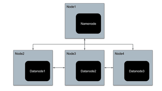
HDFS has a master-slave architecture where the master node is called NameNode and slave node is called DataNode. The NameNode and its DataNodes form a cluster. NameNode acts like an instructor to DataNode while the DataNodes store the actual data.

source: Hasura

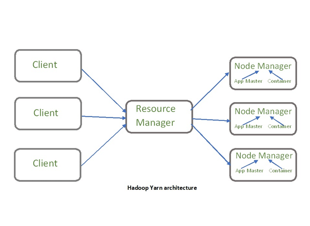
There is another component of Hadoop known as YARN. The idea of Yarn is to manage the resources and schedule/monitor jobs in Hadoop. Yarn has two main components, Resource Manager and Node Manager. The resource manager has the authority to allocate resources to various applications running in a cluster. The node manager is responsible for monitoring their resource usage (CPU, memory, disk) and reporting the same to the resource manager.

source: GeeksforGeeks

 

To understand the Hadoop architecture in detail, refer this blog –

 

Advantages of Hadoop

 

1. Economical – Hadoop is an open source Apache product, so it is free software. It has hardware cost associated with it. It is cost effective as it uses commodity hardware that are cheap machines to store its datasets and not any specialized machine.

2. Scalable – Hadoop distributes large data sets across multiple machines of a cluster. New machines can be easily added to the nodes of a cluster and can scale to thousands of nodes storing thousands of terabytes of data.

3. Fault Tolerance – Hadoop, by default, stores 3 replicas of data across the nodes of a cluster. So if any node goes down, data can be retrieved from other nodes.

4. Fast – Since Hadoop processes distributed data parallelly, it can process large data sets much faster than the traditional systems. It is highly suitable for batch processing of data.

5. Flexibility – Hadoop can store structured, semi-structured as well as unstructured data. It can accept data in the form of textfile, images, CSV files, XML files, emails, etc

6. Data Locality – Traditionally, to process the data, the data was fetched from the location it is stored, to the location where the application is submitted; however, in Hadoop, the processing application goes to the location of data to perform computation. This reduces the delay in processing of data.

7. Compatibility – Most of the emerging big data tools can be easily integrated with Hadoop like Spark. They use Hadoop as a storage platform and work as its processing system.

 

Hadoop Deployment Methods

 

1. Standalone Mode – It is the default mode of configuration of Hadoop. It doesn’t use hdfs instead, it uses a local file system for both input and output. It is useful for debugging and testing.

2. Pseudo-Distributed Mode – It is also called a single node cluster where both NameNode and DataNode resides in the same machine. All the daemons run on the same machine in this mode. It produces a fully functioning cluster on a single machine.

3. Fully Distributed Mode – Hadoop runs on multiple nodes wherein there are separate nodes for master and slave daemons. The data is distributed among a cluster of machines providing a production environment.

 

Hadoop Installation on Windows 10

 

As a beginner, you might feel reluctant in performing cloud computing which requires subscriptions. While you can install a virtual machine as well in your system, it requires allocation of a large amount of RAM for it to function smoothly else it would hang constantly.

You can install Hadoop in your system as well which would be a feasible way to learn Hadoop.

We will be installing single node pseudo-distributed hadoop cluster on windows 10.

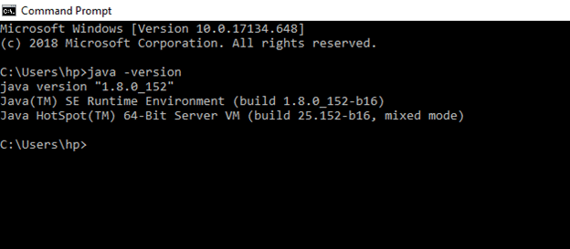
Prerequisite: To install Hadoop, you should have Java version 1.8 in your system.

Check your java version through this command on command prompt

1	java –version

 

If java is not installed in your system, then –

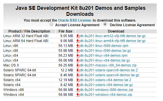
Go this link –

https://www.oracle.com/technetwork/java/javase/downloads/jdk8-downloads-2133151.html

Accept the license,

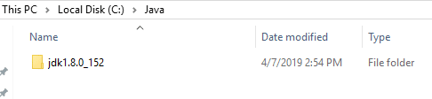
Download the file according to your operating system. Keep the java folder directly under the local disk directory (C:Javajdk1.8.0_152) rather than in Program Files (C:Program FilesJavajdk1.8.0_152) as it can create errors afterwards.

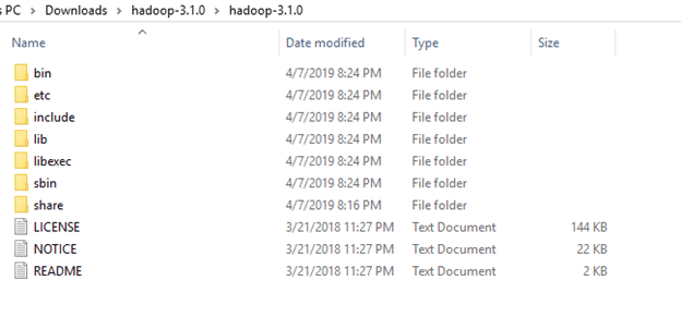
After downloading java version 1.8, download hadoop version 3.1 from this link –

https://archive.apache.org/dist/hadoop/common/hadoop-3.1.0/hadoop-3.1.0.tar.gz

Extract it to a folder.

Setup System Environment Variables

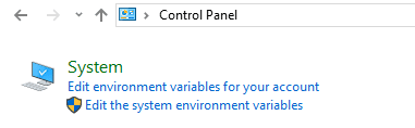
Open control panel to edit the system environment variable

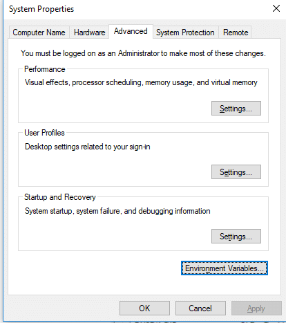
Go to environment variable in system properties

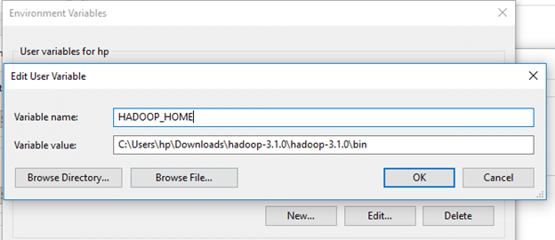
Create a new user variable. Put the Variable_name as HADOOP_HOME and Variable_value as the path of the bin folder where you extracted hadoop.

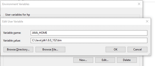
Likewise, create a new user variable with variable name as JAVA_HOME and variable value as the path of the bin folder in the Java directory.

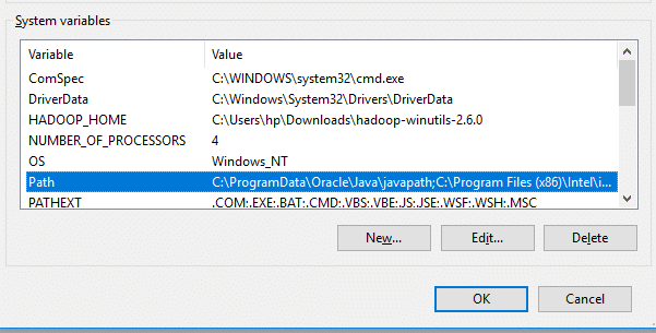
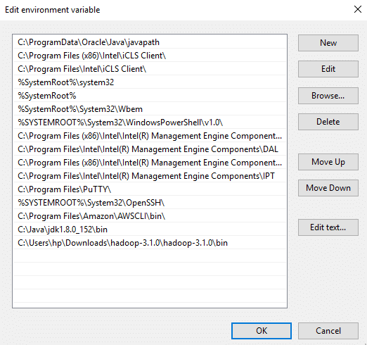
Now we need to set Hadoop bin directory and Java bin directory path in system variable path.

Edit Path in system variable

Click on New and add the bin directory path of Hadoop and Java in it.

Configurations

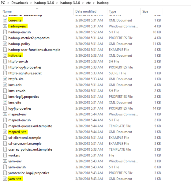
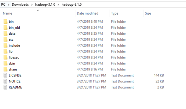
Now we need to edit some files located in the hadoop directory of the etc folder where we installed hadoop. The files that need to be edited have been highlighted.

1. Edit the file core-site.xml in the hadoop directory. Copy this xml property in the configuration in the file

1 2 3 4 5 6

<configuration>    <property>        <name>fs.defaultFS</name>        <value>hdfs://localhost:9000</value>    </property> </configuration>

 

2. Edit mapred-site.xml and copy this property in the cofiguration

1 2 3 4 5 6

<configuration>    <property>        <name>mapreduce.framework.name</name>        <value>yarn</value>    </property> </configuration>

 

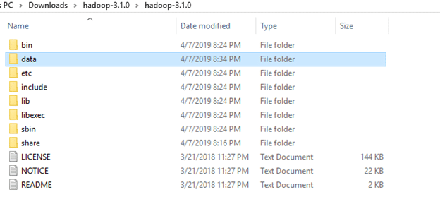
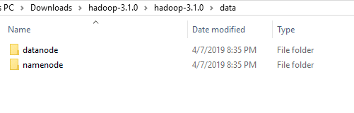
3. Create a folder ‘data’ in the hadoop directory

 

Create a folder with the name ‘datanode’ and a folder ‘namenode’ in this data directory

 

4. Edit the file hdfs-site.xml and add below property in the configuration

Note: The path of namenode and datanode across value would be the path of the datanode and namenode folders you just created.

1 2 3 4 5 6 7 8 9 10 11 12 13 14

<configuration>    <property>        <name>dfs.replication</name>        <value>1</value>    </property>    <property>        <name>dfs.namenode.name.dir</name>        <value>C:UsershpDownloadshadoop–3.1.0hadoop–3.1.0datanamenode</value>    </property>    <property>        <name>dfs.datanode.data.dir</name>        <value> C:UsershpDownloadshadoop–3.1.0hadoop–3.1.0datadatanode</value>    </property> </configuration>

 

5. Edit the file yarn-site.xml and add below property in the configuration

1 2 3 4 5 6 7 8 9 10

<configuration>    <property>      <name>yarn.nodemanager.aux–services</name>      <value>mapreduce_shuffle</value>    </property>    <property>        <name>yarn.nodemanager.auxservices.mapreduce.shuffle.class</name>   <value>org.apache.hadoop.mapred.ShuffleHandler</value>    </property> </configuration>

 

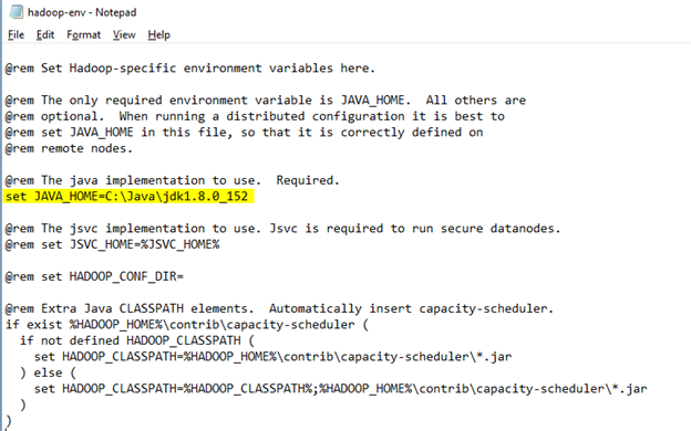
6. Edit hadoop-env.cmd and replace %JAVA_HOME% with the path of the java folder where your jdk 1.8 is installed

Hadoop needs windows OS specific files which does not come with default download of hadoop.

To include those files, replace the bin folder in hadoop directory with the bin folder provided in this github link.

https://github.com/s911415/apache-hadoop-3.1.0-winutils

Download it as zip file. Extract it and copy the bin folder in it. If you want to save the old bin folder, rename it like bin_old and paste the copied bin folder in that directory.

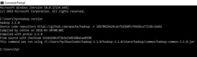
Check whether hadoop is successfully installed by running this command on cmd-

1	hadoop version

 

 

Since it doesn’t throw error and successfully shows the hadoop version, that means hadoop is successfully installed in the system.

 

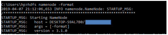
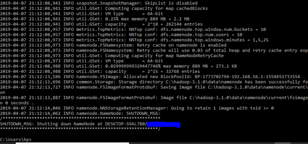
Format the NameNode

 

Formatting the NameNode is done once when hadoop is installed and not for running hadoop filesystem, else it will delete all the data inside HDFS. Run this command-

1	hdfs namenode –format

It would appear something like this –

 

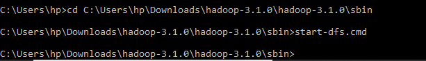
Now change the directory in cmd to sbin folder of hadoop directory with this command,

(Note: Make sure you are writing the path as per your system)

1	cd C:UsershpDownloadshadoop–3.1.0hadoop–3.1.0sbin

Start namenode and datanode with this command –

1	start–dfs.cmd

 

 

Two more cmd windows will open for NameNode and DataNode

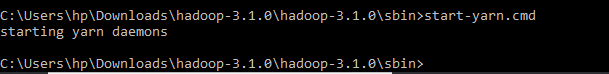
Now start yarn through this command-

1	start–yarn.cmd

 

 

Two more windows will open, one for yarn resource manager and one for yarn node manager.

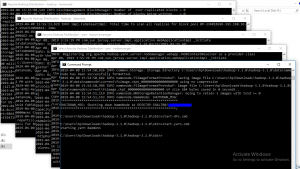
Note: Make sure all the 4 Apache Hadoop Distribution windows are up n running. If they are not running, you will see an error or a shutdown message. In that case, you need to debug the error.

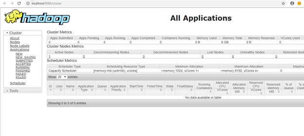
To access information about resource manager current jobs, successful and failed jobs, go to this link in browser-

http://localhost:8088/cluster

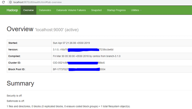
To check the details about the hdfs (namenode and datanode),

Open this link on browser-

http://localhost:9870/

Note: If you are using Hadoop version prior to 3.0.0 – Alpha 1, then use port http://localhost:50070/

 

Working with HDFS

I will be using a small text file in my local file system. To put it in hdfs using hdfs command line tool.

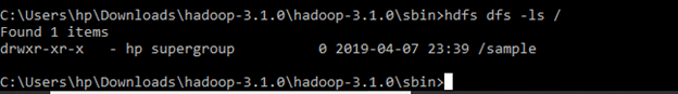
I will create a directory named ‘sample’ in my hadoop directory using the following command-

1	hdfs dfs –mkdir /sample

 

 

To verify if the directory is created in hdfs, we will use ‘ls’ command which will list the files present in hdfs –

1	hdfs dfs –ls /

 

 

Then I will copy a text file named ‘potatoes’ from my local file system to this folder that I just created in hdfs using copyFromLocal command-

1	hdfs dfs –copyFromLocal C:UsershpDownloadspotatoes.txt /sample

 

 

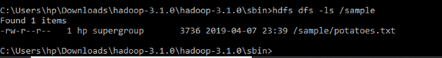
To verify if the file is copied to the folder, I will use ‘ls’ command by specifying the folder name which will read the list of files in that folder –

1	hdfs dfs –ls /sample

 

 

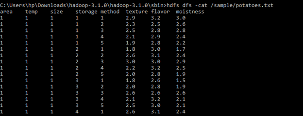
To view the contents of the file we copied, I will use cat command-

1	hdfs dfs –cat /sample/potatoes.txt

 

 

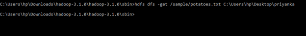
To Copy file from hdfs to local directory, I will use get command –

1	hdfs dfs –get /sample/potatoes.txt C:UsershpDesktoppriyanka

 

 

These were some basic hadoop commands. You can refer to this HDFS commands guide to learn more.

https://hadoop.apache.org/docs/r3.1.0/hadoop-project-dist/hadoop-hdfs/HDFSCommands.html

Hadoop MapReduce can be used to perform data processing activity. However, it possessed limitations due to which frameworks like Spark and Pig emerged and have gained popularity. A 200 lines of MapReduce code can be written with less than 10 lines of Pig code. Hadoop has various other components in its ecosystem like Hive, Sqoop, Oozie, and HBase. You can download these software as well in your windows system to perform data processing operations using cmd.

Follow this link, if you are looking to learn more about data science online.