Month: January 2021

MMS • RSS
Article originally posted on Data Science Central. Visit Data Science Central

AI is only used in large field lands, implementation of AI in the smaller land with lesser investment is predicted to create more growth opportunity in the forecast period. For instance, India joins GPAI as founding member to support human-centric development with the help of AI in various field including agriculture, education, finance and telecommunication. The initiative will be helpful for diversity, innovation, and economic growth of the country. During this unpredicted situation, we are helping our clients in understanding the impact of COVID19 on the global artificial intelligence in agriculture market. Our report includes:
- Technological Impact
- Social Impact
- Investment Opportunity Analysis
- Pre- & Post-COVID Market Scenario
- Infrastructure Analysis
- Supply Side & Demand Side Impact
Check out How COVID-19 impact on the Artificial Intelligence in Agriculture Market @ https://www.researchdive.com/connect-to-analyst/224
The global market is classified on the basis of application and deployment. The report offers the complete information about drivers, opportunities, restraints, segmental analysis and major players of the global market.
Factors Affecting the Market Growth
As per our analyst, increasing adoption of AI in agriculture field through sensor is predicted to be the major driving factor for the market in the forecast period. On the other hand, Lack of awareness among the farmer and the cost involved in implementing of AI in agriculture is very high which is predicted to hamper the market in the forecast period.
Drone Analytics Segment is Predicted to be the Most Profitable Segment
On the basis of application, the global artificial intelligence in agriculture market is segmented into weather tracking, precision farming, and drone analytics. Drone analytics is predicted to have the maximum market share in the forecast period. With the help of drone one can easily monitor the agricultural operation, increase crop production and optimize the agricultural activities due to which it is predicted to boost the segment market in the forecast period.
Download Sample Report of the Artificial Intelligence in Agriculture Market @ https://www.researchdive.com/request-toc-and-sample/224
Cloud Segment is Predicted to Grow Enormously
On the basis of deployment, the global artificial intelligence in agriculture market is segmented cloud, on premise, and hybrid. Cloud segment is predicted to have the highest market share in the forecast period. Cloud gives the option to the farmer to choose the right crop, cultivating process and operational activities that are associated with the respective farm which is predicted to drive the market in the forecast period.
Europe Region Market is Predicted to be the Most Profitable Region
On the basis of region, the global artificial intelligence in agriculture market is segmented North America, Asia Pacific, LAMEA, and Europe. Europe is predicted to have the highest market share in the forecast period. Increasing demand towards AI in farming and implementation of various AI techniques in farming is predicted to be the major driving factor for the global artificial intelligence in agriculture market in the forecast period.
Top Player in the Global Artificial Intelligence Market
The key players operating in the global artificial intelligence market include
- GAMAYA, Inc,
- Aerial Systems Inc.,
- aWhere Inc.
- INTERNATIONAL BUSINESS MACHINES CORPORATION,
- Farmers Edge Inc.,
- Descartes Labs, Inc.,
- Microsoft,
- Deere & Company,
- Granular, Inc.,
- The Climate Corporation
About Us:
Research Dive is a market research firm based in Pune, India. Maintaining the integrity and authenticity of the services, the firm provides the services that are solely based on its exclusive data model, compelled by the 360-degree research methodology, which guarantees comprehensive and accurate analysis. With unprecedented access to several paid data resources, team of expert researchers, and strict work ethic, the firm offers insights that are extremely precise and reliable. Scrutinizing relevant news releases, government publications, decades of trade data, and technical & white papers, Research dive deliver the required services to its clients well within the required timeframe. Its expertise is focused on examining niche markets, targeting its major driving factors, and spotting threatening hindrances. Complementarily, it also has a seamless collaboration with the major industry aficionado that further offers its research an edge.
Contact us:
Mr. Abhishek Paliwal
Research Dive
30 Wall St. 8th Floor, New York
NY 10005 (P)
+ 91 (788) 802-9103 (India)
+1 (917) 444-1262 (US)
Toll Free: +1-888-961-4454
E-mail: support@researchdive.com
LinkedIn: https://www.linkedin.com/company/research-dive/
Twitter: https://twitter.com/ResearchDive
Facebook: https://www.facebook.com/Research-Dive-1385542314927521
Blog: https://www.researchdive.com/blog
Follow us: https://marketinsightinformation.blogspot.com/
MMS • Bruno Couriol
Article originally posted on InfoQ. Visit InfoQ

The Raspberry Pi Foundation recently released the Raspberry Pi Pico, a small (21mm x 51mm), inexpensive ($4) micro-controller board based on a custom-designed RP2040 chip. The Pico can be programmed in C and MicroPython via USB. The RP2040 has two ARM cores clocking at 133MHz, 264KB internal SRAM, and 2MB QSPI Flash to connect external memories. The Pico enables a large range of applications by providing a wide range of flexible I/O options (I2C, SPI, PWM, 8 Programmable I/O state machines for custom peripheral support).
The Raspberry PI foundation described the new Pico as follows:
Raspberry Pi Pico is a tiny, fast, and versatile board built using RP2040, a brand new microcontroller chip designed by Raspberry Pi in the UK.
The Pico deserves its name with its dimensions being 21mm x 51mm. The Pico, at $4, aims to be an affordable package that can support a large range of applications. The micro-controller RP2040 features a dual-core ARM Cortex-M0+ processor, with a clock that can reach up to 133 MHz.
The versatility of the board is achieved with a large range of I/O options. The Pico exposes 26 of the 30 possible RP2040’s GPIO pins. GPIO0 to GPIO22 are digital-only. GPIO 26-28 are able to be used either as digital GPIO or as ADC inputs. The RP2040 features two UARTs, two SPI controllers, two I2C controllers, 16 PWM channels, one USB 1.1 controller, and 8 Programmable I/O (PIO) state machines.
The large range of support of communication protocols allows interfacing the Pico with plenty of available sensors and actuators. SPI is, for instance, commonly used by RFID card reader modules or 2.4 GHz wireless transmitter/receivers. I2C (Inter-Integrated Circuit communications) can be used by temperature sensors, accelerometers, magnetometers, and more. PWM (Pulse Width Modulation) can be used to control analog devices such as servomotors. The programmable state machines go a step further by allowing the implementation of custom communication protocols without involving the CPU.
The importance of versatility in Pico’s design as a differential point in the Pi’s product line is further reinforced by James Adams:
Many of our favorite projects […] connect Raspberry Pi to the physical world: software running on the Raspberry Pi reads sensors, performs computations, talks to the network, and drives actuators. […]
But there are limits: even in its lowest power mode a Raspberry Pi Zero will consume on the order of 100 milliwatts; Raspberry Pi on its own does not support analog input; and while it is possible to run “bare metal” software on a Raspberry Pi, software running under a general-purpose operating system like Linux is not well suited to low-latency control of individual I/O pins.
Reprogramming the Pico Flash can be done using a USB. Dragging a special ‘.uf2’ file onto the disk will write this file to the Flash and restart the Pico. Code may be executed directly from external memory through a dedicated SPI, DSPI, or QSPI interface. A small cache improves performance for typical applications. The Serial Wire Debug (SWD) port can be used to interactively debug code running on the RP2040.
The Pico can be programmed in C or MicroPython (written in C99). The Raspberry PI foundation provides a C/C++ SDK and an official MicroPython port. The Pico embeds additionally an on-chip clock, temperature sensor, and a single LED.
The versatility, size, and inexpensive profile of the Pico may make it attractive for embedded IoT applications. Tomas Morava, founder of the Hardwario IoT device manufacturer, previously provided actual examples of inexpensive computing devices used for industrial IoT applications. Peter Hoodie, co-founder of Moddable, which focuses on applications leveraging low-cost micro-controllers, explained in an interview with InfoQ:
Our focus on low-end microcontrollers is one example of focus on the product owner. We want to see great software – secure, reliable, easy-to-use software – on every device. That isn’t going to happen if the product requires a hundred dollars worth of hardware to run the software.
Raspberry Pi is a series of small single-board computers developed in the United Kingdom by the Raspberry Pi Foundation to promote the teaching of basic computer science in schools and in developing countries.
MMS • RSS
Article originally posted on Data Science Central. Visit Data Science Central

The Mechanical Unrest, the time frame in which agrarian and workmanship economies moved quickly to modern and machine-producing overwhelmed ones, started in the Assembled Realm in the eighteenth century and later spread all through numerous different pieces of the world. This monetary change changed not just how work was done and merchandise were delivered, yet it likewise adjusted how individuals related both to each other and to the planet on the loose.
This discount change in cultural association proceeds with today, and it has delivered a few impacts that have undulated all through Earth’s political, natural, and social circles. The accompanying rundown portrays a portion of the extraordinary advantages just as a portion of the huge deficiencies related with the Mechanical Insurgency.
Pros
Products Turned out to be More Moderate and More Available
Plants and the machines that they housed started to deliver things quicker and less expensive than could be made by hand. As the stockpile of different things rose, their expense to the buyer declined (see organic market). Shoes, dress, family products, instruments, and different things that upgrade individuals’ personal satisfaction turned out to be more normal and more affordable. Unfamiliar business sectors additionally were made for these products, and the equilibrium of exchange moved for the maker—which carried expanded abundance to the organizations that created these merchandise and added charge income to government coffers. Notwithstanding, it additionally added to the abundance imbalance between merchandise creating and products devouring nations.
The Quick Advancement of Work Saving Creations
The fast creation of hand instruments and other helpful things prompted the improvement of new kinds of apparatuses and vehicles to convey products and individuals starting with one spot then onto the next. The development of street and rail transportation and the creation of the message during The Industrial Revolution (and its related foundation of transmit—and later phone and fiber optic—lines) implied that expression of advances in assembling, agrarian gathering, energy creation, and clinical methods could be imparted between invested individuals rapidly. Work saving machines, for example, the turning jenny (a different shaft machine for turning fleece or cotton) and different creations, particularly those determined by power, (for example, home apparatuses and refrigeration) and non-renewable energy sources, (for example, autos and other fuel-controlled vehicles), are likewise notable results of the Modern Upset.
The Quick Development of Medication
The Mechanical Insurgency was the motor behind different advances in medication. Industrialization permitted clinical instruments, (for example, surgical tools, magnifying lens focal points, test tubes, and other hardware) to be created all the more rapidly. Utilizing machine fabricating, refinements to these instruments could all the more proficiently turn out to the doctors that required them. As correspondence between doctors in various zones improved, the subtleties behind new fixes and medicines for illness could be scattered rapidly, bringing about better consideration.
Improved Riches and Personal satisfaction of the Normal Individual
Large scale manufacturing brought down the expenses of much-required devices, garments, and other family unit things for the normal (that is, nonaristocratic) individuals, which permitted them to set aside cash for different things and assemble individual riches. Also, as new assembling machines were developed and new production lines were fabricated, new work openings emerged. Never again was the normal individual so intently attached to land-related concerns, (for example, being reliant upon the wages ranch work could give or the plant and animal items homesteads could create). Industrialization decreased the accentuation on landownership as the main wellspring of individual abundance. The rising interest for fabricated products implied that normal individuals could make their fortunes in urban communities as processing plant workers and as representatives of organizations that upheld the industrial facilities, which paid preferred wages over homestead related positions.
The Ascent of Expert Callings
As industrialization advanced, increasingly more country people rushed to the urban areas looking for better compensation in the processing plants. To build the plants’ general effectiveness and to make the most of new chances on the lookout, assembly line laborers were prepared to perform particular undertakings. Production line proprietors partitioned their laborers into various gatherings, each gathering zeroing in on a particular errand. A few gatherings made sure about and moved to the plants crude materials (specifically iron, coal, and steel) utilized in large scale manufacturing of merchandise, while different gatherings worked various machines. A few gatherings of laborers fixed machines when they separated, while others were accused of making upgrades to them and by and large production line activity.
Con
Congestion of Urban areas and Mechanical Towns
The guarantee of better wages pulled in travelers to urban areas and modern towns that were badly set up to deal with them. Albeit introductory lodging deficiencies in numerous zones in the end offered approach to development blasts and the advancement of current structures, squeezed shantytowns comprised of shacks and different types of low quality lodging showed up first. Nearby sewerage and sterilization frameworks were overpowered by the abrupt convergence of individuals, and drinking water was regularly defiled. Individuals living in such closeness, exhausted by helpless working conditions, and drinking perilous water introduced ideal conditions for episodes of typhus, cholera, smallpox, tuberculosis, and other irresistible illnesses. The need to treat these and different sicknesses in metropolitan regions prodded clinical advances and the improvement of present day building regulations, wellbeing laws, and metropolitan arranging in many industrialized urban communities.
Contamination and Other Ecological Ills
With generally couple of special cases, the world’s advanced ecological issues started or were incredibly exacerbated by the Modern Insurgency. To fuel the industrial facilities and to support the yield of every single sort of made great, normal assets (water, trees, soil, rocks and minerals, wild and tamed creatures, and so forth) were changed, which decreased the planet’s load of significant regular capital. The worldwide difficulties of far and wide water and air contamination, decreases in biodiversity, decimation of untamed life natural surroundings, and even a dangerous atmospheric devation can be followed back to this crossroads in mankind’s set of experiences. The more nations industrialize in quest for their own riches, the more prominent this environmental change becomes.
Helpless Working Conditions
At the point when processing plants jumped up in the urban areas and modern towns, their proprietors valued creation and benefit over all else. Specialist wellbeing and wages were less significant. Assembly line laborers procured more prominent wages contrasted and horticultural specialists, yet this frequently came to the detriment of time and not exactly ideal working conditions. Assembly line laborers regularly toiled 14–16 hours out of each day six days out of every week. Men’s small wages were regularly more than double those of ladies. The wages acquired by youngsters who attempted to enhance family pay were even lower. The different machines in the production line were frequently messy, removing smoke and residue, and hazardous, the two of which added to mishaps that brought about laborer wounds and passings.
The Ascent in Undesirable Propensities
As more modest work saving gadgets become accessible, individuals performed less exhausting actual work. While difficult homestead related work was made far simpler, and much of the time far more secure, by supplanting creature force and human force with farm haulers and other particular vehicles to work the dirt and plant and gather crops, different vehicles, for example, prepares and cars, viably diminished the measure of solid exercise individuals participated in every day. Additionally, numerous callings that necessary a lot of actual effort outperform
Conclusion
A fascinating investigation of the social-financial effects of genuine development is the advantages and disadvantages of the Mechanical Insurgency. Such a timeframe the world had seen nothing. It might never again see a supported pattern of imagination that could create such gigantic abundance.
What we can do is take a gander at the occasions of history, become familiar with the exercises that are open, and put forth a cognizant attempt to dodge the slip-ups that our progenitors made around two centuries back.
MMS • Diogo Poeira Miguel Gamboa
Article originally posted on InfoQ. Visit InfoQ

Data structures are an intrinsic part of every programming language, yet Java’s Stream interface lacks vital operations and its complex approach to extensibility gave rise to alternative libraries such as jOOλ and Guava. This article provides an alternative approach that can be easily integrated in any Java project using Kotlin’s Sequence interface.
By Diogo Poeira, Miguel Gamboa
MMS • Eran Stiller
Article originally posted on InfoQ. Visit InfoQ
![]()
In a series of blog posts published recently, BBC Online’s lead technical architect explains why BBC Online uses serverless and how they optimize for it. According to the author, BBC Online uses AWS Lambda for most of its core implementation due to its ability to scale extremely fast. When a breaking news story erupts, traffic can increase 3x in a single minute and then keep rising after that.
By Eran Stiller
MMS • RSS
Article originally posted on Data Science Central. Visit Data Science Central

Artificial intelligence (AI) is the horsepower of the future, and its importance going forward was even more emphasized due to the Covid 19 pandemic. Being valued at $27.23 billion as of 2019, the artificial intelligence market is expected to reach $267 billion globally by 2027, a 1000% increase in the space of eight years.
AI is set to have a huge impact on the sales process over the coming years with 91.5% of top businesses already having an ongoing investment in artificial intelligence. Buyer analytics provided by AI will give key insight to help get deals across the line.
How exactly is AI upending the B2B sales experience? Three major aspects are discussed below:
Optimizing processes
57% of sales reps are expected to miss quota this year. This would be largely due to inefficient and unorganized sales processes.
However, artificial intelligence is expected to facilitate great strides in the direction of sales process optimization. This would begin with sales onboarding. A study of some companies showed that onboarding of sales reps takes about 4.5 months. Some companies may even take over 7 months for new reps to get fully productive.
Using its analytical capabilities, AI will serve as a guide to new sales reps, giving them insight on how often they should reach out to a possible buyer and how to close deals efficiently. This will reduce the time it takes to onboard new reps because they are guided to taking the most effective courses of action.
AI will also play a major role in facilitating processes such as the preparation of content. This was a job normally left to the employee who could write the best essay, if there was no such person, the company made do with the best essay writing services it could find. Writing experts at Dissertation Today say that receiving such offers from companies is quite common.
Features like automation and Natural Language Processing (NLP) would make these processes much more seamless. Lesser tasks can now be automated, giving sales reps more time to focus on more productive issues. AI will allow data to be collected in one place, making it more accessible for meetings with potential buyers.
This takes us to our next point.
Automation of mundane sales tasks
Scheduling meetings are a painstaking process. More was time is spent on scheduling meetings than on the actual meetings themselves. Sales reps could spend up to 4.75 hours arranging meetings; from sending out reminders to communicating new information.
However, AI has given us automation. There are several new software that use AI-powered automation to make these processes so much easier.
AI can also help automate the tracking and acquisition of buyer data. So, the sales reps pay proper attention to the needs of the buyer.
Personalization
77% of buyers prefer a brand that offers a personalized experience. Sadly, a study by Forrester shows that nearly 8 in 10 buyers say sales reps meet them with irrelevant content.
AI brings an entirely new dimension to personalization in the B2B sales experience. This will largely affect lead scoring. As of now, lead scoring has to do with ranking leads to find out their sales-readiness. Lead scoring is done based on the level of interest showed in your business, how they factor into your business strategy, and their current position in the buying cycle. With AI managing all the data concerning marketing, buyers, and sales, things would become easier for sales reps. Sales reps will be handed information that is tailored specifically to the needs of each lead.
The amount of accurate content available to salespeople will also be dramatically affected by artificial intelligence. The Internet of Things (IoT) poses quite some interesting possibilities when you integrate the data coming from it. The main purpose of such data would be to monitor products. But it’s likely that a situation in which, for instance, Airbus, after monitoring their own products digitally, comes up with a personalized product list for Virgin America at the exact time they may be considering replacing a particular machine part on some planes in their fleet.
Wrapping it all up
The application of artificial intelligence to the B2B sales process will have a huge effect on the way sales reps work. One great benefit of using AI will be feedback generation. Data from when customers first see a product to monitoring those they later acquire can be collected and used to improve customer experience. AI will change the way sales and marketing work, bringing more efficiency and intelligence.
Artificial intelligence is still surrounded by certain myths. This may leave companies feeling skeptical about adopting this technology. However, AI is the sales rep’s best friend. It facilitates healthier and better relationships between reps and customers, thus increasing company success.
Author Bio:
Ashley Simmons is a professional journalist and editor. She has been working in a newspaper in Salt Lake City for 4 years. She is also a content writing expert on topics such as psychology, modern education, business, and marketing innovations. She is a master in her craft.
MMS • RSS
Article originally posted on Data Science Central. Visit Data Science Central

There was a time when businesses had to give index cards and other similar cards for their customers to fill as a survey. This was how they measured their success or failure in marketing. With this method, they would collect static data like names, addresses, customer satisfaction levels, items purchased, etc. They would then go ahead to sort this information and analyze it manually. It seemed effective at the time, but in reality, it was time-wasting and relatively useless (maybe due to its monotonous nature). It was impossible to get the full idea of what customers wanted and the common trends.
The introduction of Artificial Intelligence and Big Data has done a lot in this aspect. Little wonder, they’re now commonly discussed subjects. They have proven effective in understanding consumer needs and trends. This has made them very important to many businesses, and email marketers almost can’t do without them.
As far as email marketing is concerned, AI helps marketers provide customers with their exact needs. However, it’s not just AI; there’s big data as well. With big data, email marketers have every piece of information they need—combining these two means that they’re able to stay ahead of the curve and beat their competition in the marketplace.
This is such a big deal for businesses because email marketing is one of the most effective marketing channels with a very high ROI. It has been even more effective with AI and big data as they’ve completely transformed email marketing. Here’s how:
1. Predictive Analysis
The collection of big data and analysis goes a long way to give businesses insight into important details such as their customers’ buying behavior. With this insight, it becomes possible to predict the future purchases of the customers.
For instance, businesses will have insight into popularly purchased products and the customers making the purchases. So, suppose they get a new client that fits into a particular demographic and buys a specific item. In that case, they’re able to boost their post-purchase revenue by sending tailored emails to the client with an email template builder to show them other related items to the initial one they purchased.
2. Personalization
According to essay writers at online assignment help, one of the best ways to improve emails’ effectiveness is by personalizing them.
While it is possible to send out the same emails to the whole subscriber list, that’s far from effective. It would be more helpful and practical for marketers to create personalized and targeted emails for individuals or segment their email list into groups and send targeted emails to each group. This will depend on factors such as customer demographics, preferred products, location, etc.
It is well proven that sending emails to individuals who reflect their needs will quickly grab their attention and are more likely to engage it. This might be because it resonates with them.
3. Optimizing send times
The click rate and open rates of emails are strongly affected by the send time. This means that the time you send an email will determine how much the recipients open and click through the email. You must know your recipients well, and the time they’re more likely to be free and ready to open an email.
Gone are the days when email marketers send out the same emails to all their subscribers at the same time. If you want your emails to be effective, you have to send them at the right time that the individual recipients will likely open them. Thankfully, this is something that you can achieve quickly with AI.
AI also allows you to customize the rate of email messages that a particular subscriber gets based on their engagement history. The idea is for email marketers to optimize leads and customer touchpoints when they’ll likely make more conversions.
4. Optimizing subject lines
Bryan Reynolds, a digital marketer and author at essay writing reviews, had this to say about subject lines:
“The subject line is like an eye-opener. It either opens the eye of the email recipient to the content of the email and causes them to open, or it fails to accomplish its goal.”
One thing is evident when a subject line is used effectively; it will accomplish its goal – which is to get people to read the email.
Creating a perfect subject line is something that email marketers have struggled with for many years. The introduction of AI means that it is easier to use the right subject lines, call-to-action, body copy, etc., in an email to increase open rates. Companies now know why their customers read their emails and what they have to incorporate into them.
Conclusion
Big data and AI will only get better as the years go by. So, the sooner businesses can jump on it to improve their email marketing campaigns, the better for them. Ordinarily, you can’t underestimate the power of email marketing, but adding AI and Big Data to it takes it to a new dimension.
Author Bio:
Ashley Simmons is a professional journalist and editor. She has been working in a newspaper in Salt Lake City for four years. She is also a content writing expert in such topics as psychology, modern education, business, and marketing innovations. She is a master in her craft.
MMS • Jessica DeVita Nick Stenning
Article originally posted on InfoQ. Visit InfoQ

Jessica DeVita (Netflix) and Nick Stenning (Microsoft) have been working on improving how software teams learn from incidents in production. In this article, they share some of what they’ve learned from the research community in this area, and offer some advice on the practical application of this work.
By Jessica DeVita, Nick Stenning
Google Updates Its Cloud Run Service Support for Websockets, Http/2, and Grpc Bidirectional Streams
MMS • Steef-Jan Wiggers
Article originally posted on InfoQ. Visit InfoQ

Cloud Run is a managed compute platform that enables developers to run stateless containers invocable via web requests or Pub/Sub events. It is serverless, meaning all infrastructure management is abstract away, and developers can focus more on building applications.
By Steef-Jan Wiggers
NLP with Bangla: word2vec, generating Bangla text & sentiment analysis (LSTM), ChatBot (RASA NLU)
MMS • RSS
Article originally posted on Data Science Central. Visit Data Science Central

In this blog, we shall discuss on a few NLP techniques with Bangla language. We shall start with a demonstration on how to train a word2vec model with Bangla wiki corpus with tensorflow and how to visualize the semantic similarity between words using t-SNE. Next, we shall demonstrate how to train a character / word LSTM on selected Tagore’s songs to generate songs like Tagore with keras.
Once that’s accomplished, we shall create sentiment analysis dataset by crawling the daily astrological prediction pages of a leading Bangla newspaper and manually labeling the sentiment of each of the predictions corresponding to each moon-sign. We shall train an LSTM sentiment a analysis model to predict the sentiment of a moon-sign prediction. Finally, we shall use RASA NLU (natural language understanding) to build a very simple chatbot in Bangla.
Word2vec model with Bangla wiki corpus with tensorflow
- Let’s start by importing the required libraries
import collections import numpy as np import tensorflow as tf from matplotlib import pylab
- Download the Bangla wikipedia corpus from Kaggle. The first few lines from the corpus are shown below:
id,text,title,url
1528,
“রবীন্দ্রনাথ ঠাকুর”
রবীন্দ্রনাথ ঠাকুর (৭ই মে, ১৮৬১ – ৭ই আগস্ট, ১৯৪১) (২৫ বৈশাখ, ১২৬৮ – ২২ শ্রাবণ, ১৩৪৮ বঙ্গাব্দ) ছিলেন অগ্রণী বাঙালি কবি, ঔপন্যাসিক, সংগীতস্রষ্টা, নাট্যকার, চিত্রকর, ছোটগল্পকার, প্রাবন্ধিক, অভিনেতা, কণ্ঠশিল্পী ও দার্শনিক। তাঁকে বাংলা ভাষার সর্বশ্রেষ্ঠ সাহিত্যিক মনে করা হয়। রবীন্দ্রনাথকে গুরুদেব, কবিগুরু ও বিশ্বকবি অভিধায় ভূষিত করা হয়। রবীন্দ্রনাথের ৫২টি কাব্যগ্রন্থ, ৩৮টি নাটক, ১৩টি উপন্যাস ও ৩৬টি প্রবন্ধ ও অন্যান্য গদ্যসংকলন তাঁর জীবদ্দশায় বা মৃত্যুর অব্যবহিত পরে প্রকাশিত হয়। তাঁর সর্বমোট ৯৫টি ছোটগল্প ও ১৯১৫টি গান যথাক্রমে “”গল্পগুচ্ছ”” ও “”গীতবিতান”” সংকলনের অন্তর্ভুক্ত হয়েছে। রবীন্দ্রনাথের যাবতীয় প্রকাশিত ও গ্রন্থাকারে অপ্রকাশিত রচনা ৩২ খণ্ডে “”রবীন্দ্র রচনাবলী”” নামে প্রকাশিত হয়েছে। রবীন্দ্রনাথের যাবতীয় পত্রসাহিত্য উনিশ খণ্ডে “”চিঠিপত্র”” ও চারটি পৃথক গ্রন্থে প্রকাশিত। এছাড়া তিনি প্রায় দুই হাজার ছবি এঁকেছিলেন। রবীন্দ্রনাথের রচনা বিশ্বের বিভিন্ন ভাষায় অনূদিত হয়েছে। ১৯১৩ সালে “”গীতাঞ্জলি”” কাব্যগ্রন্থের ইংরেজি অনুবাদের জন্য তিনি সাহিত্যে নোবেল পুরস্কার লাভ করেন।রবীন্দ্রনাথ ঠাকুর কলকাতার এক ধনাঢ্য ও সংস্কৃতিবান ব্রাহ্ম পিরালী ব্রাহ্মণ পরিবারে জন্মগ্রহণ করেন। বাল্যকালে প্রথাগত বিদ্যালয়-শিক্ষা তিনি গ্রহণ করেননি; গৃহশিক্ষক রেখে বাড়িতেই তাঁর শিক্ষার ব্যবস্থা করা হয়েছিল। আট বছর বয়সে তিনি কবিতা লেখা শুরু করেন। ১৮৭৪ সালে “”তত্ত্ববোধিনী পত্রিকা””-এ তাঁর “””” কবিতাটি প্রকাশিত হয়। এটিই ছিল তাঁর প্রথম প্রকাশিত রচনা। ১৮৭৮ সালে মাত্র সতেরো বছর বয়সে রবীন্দ্রনাথ প্রথমবার ইংল্যান্ডে যান। ১৮৮৩ সালে মৃণালিনী দেবীর সঙ্গে তাঁর বিবাহ হয়। ১৮৯০ সাল থেকে রবীন্দ্রনাথ পূর্ববঙ্গের শিলাইদহের জমিদারি এস্টেটে বসবাস শুরু করেন। ১৯০১ সালে তিনি পশ্চিমবঙ্গের শান্তিনিকেতনে ব্রহ্মচর্যাশ্রম প্রতিষ্ঠা করেন এবং সেখানেই পাকাপাকিভাবে বসবাস শুরু করেন। ১৯০২ সালে তাঁর পত্নীবিয়োগ হয়। ১৯০৫ সালে তিনি বঙ্গভঙ্গ-বিরোধী আন্দোলনে জড়িয়ে পড়েন। ১৯১৫ সালে ব্রিটিশ সরকার তাঁকে নাইট উপাধিতে ভূষিত করেন। কিন্তু ১৯১৯ সালে জালিয়ানওয়ালাবাগ হত্যাকাণ্ডের প্রতিবাদে তিনি সেই উপাধি ত্যাগ করেন। ১৯২১ সালে গ্রামোন্নয়নের জন্য তিনি শ্রীনিকেতন নামে একটি সংস্থা প্রতিষ্ঠা করেন। ১৯২৩ সালে আনুষ্ঠানিকভাবে বিশ্বভারতী প্রতিষ্ঠিত হয়। দীর্ঘজীবনে তিনি বহুবার বিদেশ ভ্রমণ করেন এবং সমগ্র বিশ্বে বিশ্বভ্রাতৃত্বের বাণী প্রচার করেন। ১৯৪১ সালে দীর্ঘ রোগভোগের পর কলকাতার পৈত্রিক বাসভবনেই তাঁর মৃত্যু হয়।রবীন্দ্রনাথের কাব্যসাহিত্যের বৈশিষ্ট্য ভাবগভীরতা, গীতিধর্মিতা চিত্ররূপময়তা, অধ্যাত্মচেতনা, ঐতিহ্যপ্রীতি, প্রকৃতিপ্রেম, মানবপ্রেম, স্বদেশপ্রেম, বিশ্বপ্রেম, রোম্যান্টিক সৌন্দর্যচেতনা, ভাব, ভাষা, ছন্দ ও আঙ্গিকের বৈচিত্র্য, বাস্তবচেতনা ও প্রগতিচেতনা। রবীন্দ্রনাথের গদ্যভাষাও কাব্যিক। ভারতের ধ্রুপদি ও লৌকিক সংস্কৃতি এবং পাশ্চাত্য বিজ্ঞানচেতনা ও শিল্পদর্শন তাঁর রচনায় গভীর প্রভাব বিস্তার করেছিল। কথাসাহিত্য ও প্রবন্ধের মাধ্যমে তিনি সমাজ, রাজনীতি ও রাষ্ট্রনীতি সম্পর্কে নিজ মতামত প্রকাশ করেছিলেন। সমাজকল্যাণের উপায় হিসেবে তিনি গ্রামোন্নয়ন ও গ্রামের দরিদ্র মানুষ কে শিক্ষিত করে তোলার পক্ষে মতপ্রকাশ করেন। এর পাশাপাশি সামাজিক ভেদাভেদ, অস্পৃশ্যতা, ধর্মীয় গোঁড়ামি ও ধর্মান্ধতার বিরুদ্ধেও তিনি তীব্র প্রতিবাদ জানিয়েছিলেন। রবীন্দ্রনাথের দর্শনচেতনায় ঈশ্বরের মূল হিসেবে মানব সংসারকেই নির্দিষ্ট করা হয়েছে; রবীন্দ্রনাথ দেববিগ্রহের পরিবর্তে কর্মী অর্থাৎ মানুষ ঈশ্বরের পূজার কথা বলেছিলেন। সংগীত ও নৃত্যকে তিনি শিক্ষার অপরিহার্য অঙ্গ মনে করতেন। রবীন্দ্রনাথের গান তাঁর অন্যতম শ্রেষ্ঠ কীর্তি। তাঁর রচিত “”আমার সোনার বাংলা”” ও “”জনগণমন-অধিনায়ক জয় হে”” গানদুটি যথাক্রমে গণপ্রজাতন্ত্রী বাংলাদেশ ও ভারতীয় প্রজাতন্ত্রের জাতীয় সংগীত।
জীবন.
প্রথম জীবন (১৮৬১–১৯০১).
শৈশব ও কৈশোর (১৮৬১ – ১৮৭৮).
রবীন্দ্রনাথ ঠাকুর কলকাতার জোড়াসাঁকো ঠাকুরবাড়িতে জন্মগ্রহণ করেছিলেন। তাঁর পিতা ছিলেন ব্রাহ্ম ধর্মগুরু দেবেন্দ্রনাথ ঠাকুর (১৮১৭–১৯০৫) এবং মাতা ছিলেন সারদাসুন্দরী দেবী (১৮২৬–১৮৭৫)। রবীন্দ্রনাথ ছিলেন পিতামাতার চতুর্দশ সন্তান। জোড়াসাঁকোর ঠাকুর পরিবার ছিল ব্রাহ্ম আদিধর্ম মতবাদের প্রবক্তা। রবীন্দ্রনাথের পূর্ব পুরুষেরা খুলনা জেলার রূপসা উপজেলা পিঠাভোগে বাস করতেন। ১৮৭৫ সালে মাত্র চোদ্দ বছর বয়সে রবীন্দ্রনাথের মাতৃবিয়োগ ঘটে। পিতা দেবেন্দ্রনাথ দেশভ্রমণের নেশায় বছরের অধিকাংশ সময় কলকাতার বাইরে অতিবাহিত করতেন। তাই ধনাঢ্য পরিবারের সন্তান হয়েও রবীন্দ্রনাথের ছেলেবেলা কেটেছিল ভৃত্যদের অনুশাসনে। শৈশবে রবীন্দ্রনাথ কলকাতার ওরিয়েন্টাল সেমিনারি, নর্ম্যাল স্কুল, বেঙ্গল অ্যাকাডেমি এবং সেন্ট জেভিয়ার্স কলেজিয়েট স্কুলে কিছুদিন করে পড়াশোনা করেছিলেন। কিন্তু বিদ্যালয়-শিক্ষায় অনাগ্রহী হওয়ায় বাড়িতেই গৃহশিক্ষক রেখে তাঁর শিক্ষার ব্যবস্থা করা হয়েছিল। ছেলেবেলায় জোড়াসাঁকোর বাড়িতে অথবা বোলপুর ও পানিহাটির বাগানবাড়িতে প্রাকৃতিক পরিবেশের মধ্যে ঘুরে বেড়াতে বেশি স্বচ্ছন্দবোধ করতেন রবীন্দ্রনাথ।১৮৭৩ সালে এগারো বছর বয়সে রবীন্দ্রনাথের উপনয়ন অনুষ্ঠিত হয়েছিল। এরপর তিনি কয়েক মাসের জন্য পিতার সঙ্গে দেশভ্রমণে বের হন। প্রথমে তাঁরা আসেন শান্তিনিকেতনে। এরপর পাঞ্জাবের অমৃতসরে কিছুকাল কাটিয়ে শিখদের উপাসনা পদ্ধতি পরিদর্শন করেন। শেষে পুত্রকে নিয়ে দেবেন্দ্রনাথ যান পাঞ্জাবেরই (অধুনা ভারতের হিমাচল প্রদেশ রাজ্যে অবস্থিত) ডালহৌসি শৈলশহরের নিকট বক্রোটায়। এখানকার বক্রোটা বাংলোয় বসে রবীন্দ্রনাথ পিতার কাছ থেকে সংস্কৃত ব্যাকরণ, ইংরেজি, জ্যোতির্বিজ্ঞান, সাধারণ বিজ্ঞান ও ইতিহাসের নিয়মিত পাঠ নিতে শুরু করেন। দেবেন্দ্রনাথ তাঁকে বিশিষ্ট ব্যক্তিবর্গের জীবনী, কালিদাস রচিত ধ্রুপদি সংস্কৃত কাব্য ও নাটক এবং উপনিষদ্ পাঠেও উৎসাহিত করতেন। ১৮৭৭ সালে “”ভারতী”” পত্রিকায় তরুণ রবীন্দ্রনাথের কয়েকটি গুরুত্বপূর্ণ রচনা প্রকাশিত হয়। এগুলি হল মাইকেল মধুসূদনের “”””, “”ভানুসিংহ ঠাকুরের পদাবলী”” এবং “””” ও “””” নামে দুটি গল্প। এর মধ্যে “”ভানুসিংহ ঠাকুরের পদাবলী”” বিশেষভাবে উল্লেখযোগ্য। এই কবিতাগুলি রাধা-কৃষ্ণ বিষয়ক পদাবলির অনুকরণে “”ভানুসিংহ”” ভণিতায় রচিত। রবীন্দ্রনাথের “”ভিখারিণী”” গল্পটি (১৮৭৭) বাংলা সাহিত্যের প্রথম ছোটগল্প। ১৮৭৮ সালে প্রকাশিত হয় রবীন্দ্রনাথের প্রথম কাব্যগ্রন্থ তথা প্রথম মুদ্রিত গ্রন্থ “”কবিকাহিনী””। এছাড়া এই পর্বে তিনি রচনা করেছিলেন “””” (১৮৮২) কাব্যগ্রন্থটি। রবীন্দ্রনাথের বিখ্যাত কবিতা “””” এই কাব্যগ্রন্থের অন্তর্গত।
যৌবন (১৮৭৮-১৯০১).
১৮৭৮ সালে ব্যারিস্টারি পড়ার উদ্দেশ্যে ইংল্যান্ডে যান রবীন্দ্রনাথ। প্রথমে তিনি ব্রাইটনের একটি পাবলিক স্কুলে ভর্তি হয়েছিলেন। ১৮৭৯ সালে ইউনিভার্সিটি কলেজ লন্ডনে আইনবিদ্যা নিয়ে পড়াশোনা শুরু করেন। কিন্তু সাহিত্যচর্চার আকর্ষণে সেই পড়াশোনা তিনি সমাপ্ত করতে পারেননি। ইংল্যান্ডে থাকাকালীন শেকসপিয়র ও অন্যান্য ইংরেজ সাহিত্যিকদের রচনার সঙ্গে রবীন্দ্রনাথের পরিচয় ঘটে। এই সময় তিনি বিশেষ মনোযোগ সহকারে পাঠ করেন “”রিলিজিও মেদিচি””, “”কোরিওলেনাস”” এবং “”অ্যান্টনি অ্যান্ড ক্লিওপেট্রা””। এই সময় তাঁর ইংল্যান্ডবাসের অভিজ্ঞতার কথা “”ভারতী”” পত্রিকায় পত্রাকারে পাঠাতেন রবীন্দ্রনাথ। উক্ত পত্রিকায় এই লেখাগুলি জ্যেষ্ঠভ্রাতা দ্বিজেন্দ্রনাথ ঠাকুরের সমালোচনাসহ প্রকাশিত হত “””” নামে। ১৮৮১ সালে সেই পত্রাবলি “””” নামে গ্রন্থাকারে ছাপা হয়। এটিই ছিল রবীন্দ্রনাথের প্রথম গদ্যগ্রন্থ তথা প্রথম চলিত ভাষায় লেখা গ্রন্থ। অবশেষে ১৮৮০ সালে প্রায় দেড় বছর ইংল্যান্ডে কাটিয়ে কোনো ডিগ্রি না নিয়ে এবং ব্যারিস্টারি পড়া শুরু না করেই তিনি দেশে ফিরে আসেন।১৮৮৩ সালের ৯ ডিসেম্বর (২৪ অগ্রহায়ণ, ১২৯০ বঙ্গাব্দ) ঠাকুরবাড়ির অধস্তন কর্মচারী বেণীমাধব রায়চৌধুরীর কন্যা ভবতারিণীর সঙ্গে রবীন্দ্রনাথের বিবাহ সম্পন্ন হয়। বিবাহিত জীবনে ভবতারিণীর নামকরণ হয়েছিল মৃণালিনী দেবী (১৮৭৩–১৯০২ )। রবীন্দ্রনাথ ও মৃণালিনীর সন্তান ছিলেন পাঁচ জন: মাধুরীলতা (১৮৮৬–১৯১৮), রথীন্দ্রনাথ (১৮৮৮–১৯৬১), রেণুকা (১৮৯১–১৯০৩), মীরা (১৮৯৪–১৯৬৯) এবং শমীন্দ্রনাথ (১৮৯৬–১৯০৭)। এঁদের মধ্যে অতি অল্প বয়সেই রেণুকা ও শমীন্দ্রনাথের মৃত্যু ঘটে।১৮৯১ সাল থেকে পিতার আদেশে নদিয়া (নদিয়ার উক্ত অংশটি অধুনা বাংলাদেশের কুষ্টিয়া জেলা), পাবনা ও রাজশাহী জেলা এবং উড়িষ্যার জমিদারিগুলির তদারকি শুরু করেন রবীন্দ্রনাথ। কুষ্টিয়ার শিলাইদহের কুঠিবাড়িতে রবীন্দ্রনাথ দীর্ঘ সময় অতিবাহিত করেছিলেন। জমিদার রবীন্দ্রনাথ শিলাইদহে “”পদ্মা”” নামে একটি বিলাসবহুল পারিবারিক বজরায় চড়ে প্রজাবর্গের কাছে খাজনা আদায় ও আশীর্বাদ প্রার্থনা করতে যেতেন। গ্রামবাসীরাও তাঁর সম্মানে ভোজসভার আয়োজন করত।১৮৯০ সালে রবীন্দ্রনাথের অপর বিখ্যাত কাব্যগ্রন্থ “””” প্রকাশিত হয়। কুড়ি থেকে ত্রিশ বছর বয়সের মধ্যে তাঁর আরও কয়েকটি উল্লেখযোগ্য কাব্যগ্রন্থ ও গীতিসংকলন প্রকাশিত হয়েছিল। এগুলি হলো “”””, “”””, “”রবিচ্ছায়া””, “””” ইত্যাদি। ১৮৯১ থেকে ১৮৯৫ সাল পর্যন্ত নিজের সম্পাদিত “”সাধনা”” পত্রিকায় রবীন্দ্রনাথের বেশ কিছু উৎকৃষ্ট রচনা প্রকাশিত হয়। তাঁর সাহিত্যজীবনের এই পর্যায়টি তাই “”সাধনা পর্যায়”” নামে পরিচিত। রবীন্দ্রনাথের “”গল্পগুচ্ছ”” গ্রন্থের প্রথম চুরাশিটি গল্পের অর্ধেকই এই পর্যায়ের রচনা। এই ছোটগল্পগুলিতে তিনি বাংলার গ্রামীণ জনজীবনের এক আবেগময় ও শ্লেষাত্মক চিত্র এঁকেছিলেন।
- Preprocess the csv files with the following code using regular expressions (to get rid of punctuations). Remember we need to decode to utf-8 first, since we have unicode input files.
from glob import glob import re words = [] for f in glob('bangla/wiki/*.csv'): words += re.sub('[rn—?,;।!‘"’.:()[]…0-9]', ' ', open(f, 'rb').read().decode('utf8').strip()).split(' ') words = list(filter(lambda x: not x in ['', '-'], words)) print(len(words)) # 13964346 words[:25] #['রবীন্দ্রনাথ', # 'ঠাকুর', # 'রবীন্দ্রনাথ', # 'ঠাকুর', # '৭ই', # 'মে', # '১৮৬১', # '৭ই', # 'আগস্ট', # '১৯৪১', # '২৫', # 'বৈশাখ', # '১২৬৮', # '২২', # 'শ্রাবণ', # '১৩৪৮', # 'বঙ্গাব্দ', # 'ছিলেন', # 'অগ্রণী', # 'বাঙালি', # 'কবি', # 'ঔপন্যাসিক', # 'সংগীতস্রষ্টা', # 'নাট্যকার', # 'চিত্রকর']
- Create indices for unique words in the dataset.
vocabulary_size = 25000 def build_dataset(words): count = [['UNK', -1]] count.extend(collections.Counter(words).most_common(vocabulary_size - 1)) dictionary = dict() for word, _ in count: dictionary[word] = len(dictionary) data = list() unk_count = 0 for word in words: if word in dictionary: index = dictionary[word] else: index = 0 # dictionary['UNK'] unk_count = unk_count + 1 data.append(index) count[0][1] = unk_count reverse_dictionary = dict(zip(dictionary.values(), dictionary.keys())) return data, count, dictionary, reverse_dictionary data, count, dictionary, reverse_dictionary = build_dataset(words) print('Most common words (+UNK)', count[:5]) # Most common words (+UNK) [['UNK', 1961151], ('এবং', 196916), ('ও', 180042), ('হয়', 160533), ('করে', 131206)] print('Sample data', data[:10]) #Sample data [1733, 1868, 1733, 1868, 5769, 287, 6855, 5769, 400, 2570] del words # Hint to reduce memory.
- Generate batches to be trained with the word2vec skip-gram model.
- The target label should be at the center of the buffer each time. That is, given a focus word, our goal will be to learn the most probable context words.
- The input and the target vector will depend on num_skips and skip_window.
data_index = 0 def generate_batch(batch_size, num_skips, skip_window): global data_index assert batch_size % num_skips == 0 assert num_skips <= 2 * skip_window batch = np.ndarray(shape=(batch_size), dtype=np.int32) labels = np.ndarray(shape=(batch_size, 1), dtype=np.int32) span = 2 * skip_window + 1 # [ skip_window target skip_window ] buffer = collections.deque(maxlen=span) for _ in range(span): buffer.append(data[data_index]) data_index = (data_index + 1) % len(data) for i in range(batch_size // num_skips): target = skip_window # targets_to_avoid = [ skip_window ] for j in range(num_skips): while target in targets_to_avoid: target = random.randint(0, span - 1) targets_to_avoid.append(target) batch[i * num_skips + j] = buffer[skip_window] labels[i * num_skips + j, 0] = buffer[target] buffer.append(data[data_index]) data_index = (data_index + 1) % len(data) return batch, labels print('data:', [reverse_dictionary[di] for di in data[:8]]) # data: ['রবীন্দ্রনাথ', 'ঠাকুর', 'রবীন্দ্রনাথ', 'ঠাকুর', '৭ই', 'মে', '১৮৬১', '৭ই'] for num_skips, skip_window in [(2, 1), (4, 2)]: data_index = 0 batch, labels = generate_batch(batch_size=8, num_skips=num_skips, skip_window=skip_window) print('nwith num_skips = %d and skip_window = %d:' % (num_skips, skip_window)) print(' batch:', [reverse_dictionary[bi] for bi in batch]) print(' labels:', [reverse_dictionary[li] for li in labels.reshape(8)]) # data: ['রবীন্দ্রনাথ', 'ঠাকুর', 'রবীন্দ্রনাথ', 'ঠাকুর', '৭ই', 'মে', '১৮৬১', '৭ই'] # with num_skips = 2 and skip_window = 1: # batch: ['ঠাকুর', 'ঠাকুর', 'রবীন্দ্রনাথ', 'রবীন্দ্রনাথ', 'ঠাকুর', 'ঠাকুর', '৭ই', '৭ই'] # labels: ['রবীন্দ্রনাথ', 'রবীন্দ্রনাথ', 'ঠাকুর', 'ঠাকুর', '৭ই', 'রবীন্দ্রনাথ', 'ঠাকুর', 'মে'] # with num_skips = 4 and skip_window = 2: # batch: ['রবীন্দ্রনাথ', 'রবীন্দ্রনাথ', 'রবীন্দ্রনাথ', 'রবীন্দ্রনাথ', 'ঠাকুর', 'ঠাকুর', 'ঠাকুর', 'ঠাকুর'] # labels: ['রবীন্দ্রনাথ', '৭ই', 'ঠাকুর', 'ঠাকুর', 'মে', 'ঠাকুর', 'রবীন্দ্রনাথ', '৭ই']
- Pick a random validation set to sample nearest neighbors.
- Limit the validation samples to the words that have a low numeric ID, which by construction are also the most frequent.
- Look up embeddings for inputs and compute the softmax loss, using a sample of the negative labels each time (this is known as negative sampling, which is used to make the computation efficient, since the number of labels are often too high).
- The optimizer will optimize the softmax_weights and the embeddings.
This is because the embeddings are defined as a variable quantity and the optimizer’s `minimize` method will by default modify all variable quantities that contribute to the tensor it is passed. - Compute the similarity between minibatch examples and all embeddings.
batch_size = 128 embedding_size = 128 # Dimension of the embedding vector. skip_window = 1 # How many words to consider left and right. num_skips = 2 # #times to reuse an input to generate a label. valid_size = 16 # Random set of words to evaluate similarity on. valid_window = 100 # Only pick dev samples in the head of the # distribution. valid_examples = np.array(random.sample(range(valid_window), valid_size)) num_sampled = 64 # Number of negative examples to sample. graph = tf.Graph() with graph.as_default(), tf.device('/cpu:0'): # Input data. train_dataset = tf.placeholder(tf.int32, shape=[batch_size]) train_labels = tf.placeholder(tf.int32, shape=[batch_size, 1]) valid_dataset = tf.constant(valid_examples, dtype=tf.int32) # Variables. embeddings = tf.Variable( tf.random_uniform([vocabulary_size, embedding_size], -1.0, 1.0)) softmax_weights = tf.Variable( tf.truncated_normal([vocabulary_size, embedding_size], stddev=1.0 / math.sqrt(embedding_size))) softmax_biases = tf.Variable(tf.zeros([vocabulary_size])) # Model. embed = tf.nn.embedding_lookup(embeddings, train_dataset) loss = tf.reduce_mean( tf.nn.sampled_softmax_loss(weights=softmax_weights, biases=softmax_biases, inputs=embed, labels=train_labels, num_sampled=num_sampled, num_classes=vocabulary_size)) # Optimizer. optimizer = tf.train.AdagradOptimizer(1.0).minimize(loss) # use the cosine distance: norm = tf.sqrt(tf.reduce_sum(tf.square(embeddings), 1, keepdims=True)) normalized_embeddings = embeddings / norm valid_embeddings = tf.nn.embedding_lookup(normalized_embeddings, valid_dataset) similarity = tf.matmul(valid_embeddings, tf.transpose(normalized_embeddings))
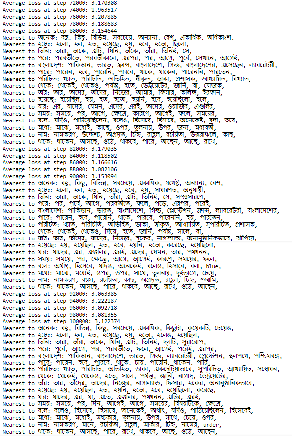
- Train the word2vec model with the batches constructed, for 100k steps.
num_steps = 100001with tf.Session(graph=graph) as session: tf.global_variables_initializer().run() print('Initialized') average_loss = 0 for step in range(num_steps): batch_data, batch_labels = generate_batch( batch_size, num_skips, skip_window) feed_dict = {train_dataset : batch_data, train_labels : batch_labels} _, l = session.run([optimizer, loss], feed_dict=feed_dict) average_loss += l if step % 2000 == 0: if step > 0: average_loss = average_loss / 2000 # The average loss is an estimate of the loss over the last # 2000 batches. print('Average loss at step %d: %f' % (step, average_loss)) average_loss = 0 # note that this is expensive (~20% slowdown if computed every # 500 steps) if step % 10000 == 0: sim = similarity.eval() for i in range(valid_size): valid_word = reverse_dictionary[valid_examples[i]] top_k = 8 # number of nearest neighbors nearest = (-sim[i, :]).argsort()[1:top_k+1] log = 'Nearest to %s:' % valid_word for k in range(top_k): close_word = reverse_dictionary[nearest[k]] log = '%s %s,' % (log, close_word) print(log) final_embeddings = normalized_embeddings.eval()
- The following shows how the loss function decreases with the increase in training steps.
- During the training process, the words that become semantically near come closer in the embedding space.
- Use t-SNE plot to map the following words from 128-dimensional embedding space to 2 dimensional manifold and visualize.
words = ['রাজা', 'রাণী', 'ভারত','বাংলাদেশ','দিল্লী','কলকাতা','ঢাকা', 'পুরুষ','নারী','দুঃখ','লেখক','কবি','কবিতা','দেশ', 'বিদেশ','লাভ','মানুষ', 'এবং', 'ও', 'গান', 'সঙ্গীত', 'বাংলা', 'ইংরেজি', 'ভাষা', 'কাজ', 'অনেক', 'জেলার', 'বাংলাদেশের', 'এক', 'দুই', 'তিন', 'চার', 'পাঁচ', 'দশ', '১', '৫', '২০', 'নবম', 'ভাষার', '১২', 'হিসাবে', 'যদি', 'পান', 'শহরের', 'দল', 'যদিও', 'বলেন', 'রান', 'করেছে', 'করে', 'এই', 'করেন', 'তিনি', 'একটি', 'থেকে', 'করা', 'সালে', 'এর', 'যেমন', 'সব', 'তার', 'খেলা', 'অংশ', 'উপর', 'পরে', 'ফলে', 'ভূমিকা', 'গঠন', 'তা', 'দেন', 'জীবন', 'যেখানে', 'খান', 'এতে', 'ঘটে', 'আগে', 'ধরনের', 'নেন', 'করতেন', 'তাকে', 'আর', 'যার', 'দেখা', 'বছরের', 'উপজেলা', 'থাকেন', 'রাজনৈতিক', 'মূলত', 'এমন', 'কিলোমিটার', 'পরিচালনা', '২০১১', 'তারা', 'তিনি', 'যিনি', 'আমি', 'তুমি', 'আপনি', 'লেখিকা', 'সুখ', 'বেদনা', 'মাস', 'নীল', 'লাল', 'সবুজ', 'সাদা', 'আছে', 'নেই', 'ছুটি', 'ঠাকুর', 'দান', 'মণি', 'করুণা', 'মাইল', 'হিন্দু', 'মুসলমান','কথা', 'বলা', 'সেখানে', 'তখন', 'বাইরে', 'ভিতরে', 'ভগবান' ] indices = [] for word in words: #print(word, dictionary[word]) indices.append(dictionary[word]) two_d_embeddings = tsne.fit_transform(final_embeddings[indices, :]) plot(two_d_embeddings, words)
- The following figure shows how the words similar in meaning are mapped to embedding vectors that are close to each other.
- Also, note that arithmetic property of the word embeddings: e.g., the words ‘রাজা’ and ‘রাণী’ are approximately along the same distance and direction as the words ‘লেখক’ and ‘লেখিকা’, reflecting the fact that the nature of the semantic relatedness in terms of gender is same.

- The following animation shows how the embedding is learnt to preserve the semantic similarity in the 2D-manifold more and more as training proceeds.

Generating song-like texts with LSTM from Tagore’s Bangla songs
Text generation with Character LSTM
- Let’s import the required libraries first.
from tensorflow.keras.callbacks import LambdaCallback from tensorflow.keras.models import Sequential from tensorflow.keras.layers import Dense from tensorflow.keras.layers import LSTM from tensorflow.keras.optimizers import RMSprop, Adam import io, re
- Read the input file, containing few selected songs of Tagore in Bangla.
raw_text = open('rabindrasangeet.txt','rb').read().decode('utf8') print(raw_text[0:1000]) পূজা অগ্নিবীণা বাজাও তুমি অগ্নিবীণা বাজাও তুমি কেমন ক’রে ! আকাশ কাঁপে তারার আলোর গানের ঘোরে ।। তেমনি ক’রে আপন হাতে ছুঁলে আমার বেদনাতে, নূতন সৃষ্টি জাগল বুঝি জীবন-‘পরে ।। বাজে ব’লেই বাজাও তুমি সেই গরবে, ওগো প্রভু, আমার প্রাণে সকল সবে । বিষম তোমার বহ্নিঘাতে বারে বারে আমার রাতে জ্বালিয়ে দিলে নূতন তারা ব্যথায় ভ’রে ।। অচেনাকে ভয় কী অচেনাকে ভয় কী আমার ওরে? অচেনাকেই চিনে চিনে উঠবে জীবন ভরে ।। জানি জানি আমার চেনা কোনো কালেই ফুরাবে না, চিহ্নহারা পথে আমায় টানবে অচিন ডোরে ।। ছিল আমার মা অচেনা, নিল আমায় কোলে । সকল প্রেমই অচেনা গো, তাই তো হৃদয় দোলে । অচেনা এই ভুবন-মাঝে কত সুরেই হৃদয় বাজে- অচেনা এই জীবন আমার, বেড়াই তারি ঘোরে ।।অন্তর মম অন্তর মম বিকশিত করো অন্তরতর হে- নির্মল করো, উজ্জ্বল করো, সুন্দর করো হে ।। জাগ্রত করো, উদ্যত করো, নির্ভয় করো হে ।। মঙ্গল করো, নিরলস নিঃসংশয় করো হে ।। যুক্ত করো হে সবার সঙ্গে, মুক্ত করো হে বন্ধ । সঞ্চার করো সকল কর্মে শান্ত তোমার ছন্দ । চরণপদ্মে মম চিত নিস্পন্দিত করো হে । নন্দিত করো, নন্দিত করো, নন্দিত করো হে ।। অন্তরে জাগিছ অন্তর্যামী অন্তরে জাগিছ অন্তর্যামী ।
- Here we shall be using a many-to-many RNN as shown in the next figure.

- Pre-process the text and create character indices to be used as the input in the model.
processed_text = raw_text.lower() print('corpus length:', len(processed_text)) # corpus length: 207117 chars = sorted(list(set(processed_text))) print('total chars:', len(chars)) # total chars: 89 char_indices = dict((c, i) for i, c in enumerate(chars)) indices_char = dict((i, c) for i, c in enumerate(chars))
- Cut the text in semi-redundant sequences of maxlen characters.
def is_conjunction(c): h = ord(c) # print(hex(ord(c))) return (h >= 0x980 and h = 0x9bc and h = 0x9f2) maxlen = 40 step = 2 sentences = [] next_chars = [] i = 0 while i < len(processed_text) - maxlen: if is_conjunction(processed_text[i]): i += 1 continue sentences.append(processed_text[i: i + maxlen]) next_chars.append(processed_text[i + maxlen]) i += step print('nb sequences:', len(sentences)) # nb sequences: 89334
- Create one-hot-encodings.
x = np.zeros((len(sentences), maxlen, len(chars)), dtype=np.bool) y = np.zeros((len(sentences), len(chars)), dtype=np.bool) for i, sentence in enumerate(sentences): for t, char in enumerate(sentence): x[i, t, char_indices[char]] = 1 y[i, char_indices[next_chars[i]]] = 1
- Build a model, a single LSTM.
model = Sequential() model.add(LSTM(256, input_shape=(maxlen, len(chars)))) model.add(Dense(128, activation='relu')) model.add(Dense(len(chars), activation='softmax')) optimizer = Adam(lr=0.01) #RMSprop(lr=0.01) model.compile(loss='categorical_crossentropy', optimizer=optimizer)
- The following figure how the model architecture looks like:
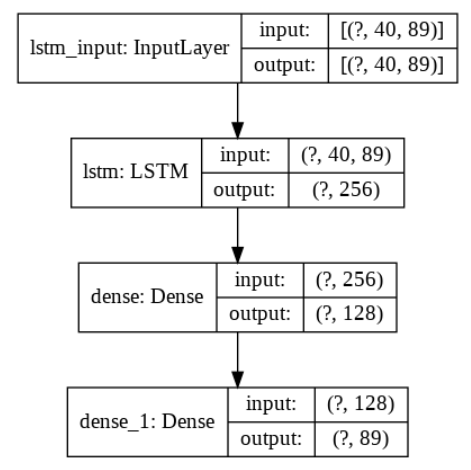
- Print the model summary.
model.summary() Model: "sequential" _________________________________________________________________ Layer (type) Output Shape Param # ================================================================= lstm (LSTM) (None, 256) 354304 _________________________________________________________________ dense (Dense) (None, 128) 32896 _________________________________________________________________ dense_1 (Dense) (None, 89) 11481 ================================================================= Total params: 398,681 Trainable params: 398,681 Non-trainable params: 0 _________________________________________________________________
- Use the following helper function to sample an index from a probability array.
def sample(preds, temperature=1.0): preds = np.asarray(preds).astype('float64') preds = np.log(preds) / temperature exp_preds = np.exp(preds) preds = exp_preds / np.sum(exp_preds) probas = np.random.multinomial(1, preds, 1) return np.argmax(probas)
- Fit the model and register a callback to print the text generated by the model at the end of each epoch.
print_callback = LambdaCallback(on_epoch_end=on_epoch_end) model.fit(x, y, batch_size=128, epochs=60, callbacks=[print_callback])
- The following animation shows how the model generates song-like texts with given seed texts, for different values of the temperature parameter.
Text Generation with Word LSTM
- Pre-process the input text, split by punctuation characters and create word indices to be used as the input in the model.
processed_text = raw_text.lower() from string import punctuation r = re.compile(r'[s{}]+'.format(re.escape(punctuation))) words = r.split(processed_text) print(len(words)) words[:16] 39481 # ['পূজা', # 'অগ্নিবীণা', # 'বাজাও', # 'তুমি', # 'অগ্নিবীণা', # 'বাজাও', # 'তুমি', # 'কেমন', # 'ক’রে', # 'আকাশ', # 'কাঁপে', # 'তারার', # 'আলোর', # 'গানের', # 'ঘোরে', # '।।'] unique_words = np.unique(words) unique_word_index = dict((c, i) for i, c in enumerate(unique_words)) index_unique_word = dict((i, c) for i, c in enumerate(unique_words))
- Create a word-window of length 5 to predict the next word.
WORD_LENGTH = 5 prev_words = [] next_words = [] for i in range(len(words) - WORD_LENGTH): prev_words.append(words[i:i + WORD_LENGTH]) next_words.append(words[i + WORD_LENGTH]) print(prev_words[1]) # ['অগ্নিবীণা', 'বাজাও', 'তুমি', 'অগ্নিবীণা', 'বাজাও'] print(next_words[1]) # তুমি print(len(unique_words)) # 7847
- Create OHE for input and output words as done for character-RNN. Fit the model on the pre-rpocessed data.
print_callback = LambdaCallback(on_epoch_end=on_epoch_end) model.fit(X, Y, batch_size=128, epochs=60, callbacks=[print_callback])
- The following animation shows the song -like text generated by the word-LSTM at the end of an epoc.

Bangla Sentiment Analysis using LSTM with Daily Astrological Prediction Dataset
- Let’s first create sentiment analysis dataset by crawling the daily astrological predictions (রাশিফল) page of the online edition of আনন্দবাজার পত্রিকা (e.g., for the year 2013), a leading Bangla newspaper and then manually labeling the sentiment of each of the predictions corresponding to each moon-sign.
- Read the csv dataset, the first few lines look like the following.
df = pd.read_csv('horo_2013_labeled.csv') pd.set_option('display.max_colwidth', 135) df.head(20)

- Transform each text in texts in a sequence of integers.
tokenizer = Tokenizer(num_words=2000, split=' ') tokenizer.fit_on_texts(df['আপনার আজকের দিনটি'].values) X = tokenizer.texts_to_sequences(df['আপনার আজকের দিনটি'].values) X = pad_sequences(X) X #array([[ 0, 0, 0, ..., 26, 375, 3], # [ 0, 0, 0, ..., 54, 8, 1], # [ 0, 0, 0, ..., 108, 42, 43], # ..., # [ 0, 0, 0, ..., 1336, 302, 82], # [ 0, 0, 0, ..., 1337, 489, 218], # [ 0, 0, 0, ..., 2, 316, 87]])
- Here we shall use a many-to-one RNN for sentiment analysis as shown below.

- Build an LSTM model that takes a sentence as input and outputs the sentiment label.
model = Sequential() model.add(Embedding(2000, 128,input_length = X.shape[1])) model.add(SpatialDropout1D(0.3)) model.add(LSTM(128, dropout=0.2, recurrent_dropout=0.2)) model.add(Dense(2,activation='softmax')) model.compile(loss = 'categorical_crossentropy', optimizer='adam',metrics = ['accuracy']) print(model.summary()) _________________________________________________________________ Layer (type) Output Shape Param # ================================================================= embedding_10 (Embedding) (None, 12, 128) 256000 _________________________________________________________________ spatial_dropout1d_10 (Spatia (None, 12, 128) 0 _________________________________________________________________ lstm_10 (LSTM) (None, 128) 131584 _________________________________________________________________ dense_10 (Dense) (None, 2) 258 ================================================================= Total params: 387,842 Trainable params: 387,842 Non-trainable params: 0 _________________________________________________________________ None
- Divide the dataset into train and validation (test) dataset and train the LSTM model on the dataset.
Y = pd.get_dummies(df['sentiment']).values X_train, X_test, Y_train, Y_test, _, indices = train_test_split(X,Y, np.arange(len(X)), test_size = 0.33, random_state = 5) model.fit(X_train, Y_train, epochs = 5, batch_size=32, verbose = 2) #Epoch 1/5 - 3s - loss: 0.6748 - acc: 0.5522 #Epoch 2/5 - 1s - loss: 0.5358 - acc: 0.7925 #Epoch 3/5 - 1s - loss: 0.2368 - acc: 0.9418 #Epoch 4/5 - 1s - loss: 0.1011 - acc: 0.9761 #Epoch 5/5 - 1s - loss: 0.0578 - acc: 0.9836
- Predict the sentiment labels of the (held out) test dataset.
result = model.predict(X[indices],batch_size=1,verbose = 2) df1 = df.iloc[indices] df1['neg_prob'] = result[:,0] df1['pos_prob'] = result[:,1] df1['pred'] = np.array(['negative', 'positive'])[np.argmax(result, axis=1)] df1.head()

- Finally, compute the accuracy of the model for the positive and negative ground-truth sentiment corresponding to daily astrological predictions.
df2 = df1[df1.sentiment == 'positive'] print('positive accuracy:' + str(np.mean(df2.sentiment == df2.pred))) #positive accuracy:0.9177215189873418 df2 = df1[df1.sentiment == 'negative'] print('negative accuracy:' + str(np.mean(df2.sentiment == df2.pred))) #negative accuracy:0.9352941176470588
Building a very simple Bangla Chatbot with RASA NLU
- The following figure shows how to design a very simple Bangla chatbot to order food from restaurants using RASA NLU.
- We need to design the intents, entities and slots to extract the entities properly and then design stories to define how the chatbot will respond to user inputs (core / dialog).
- The following figure shows how the nlu, domain and stories files are written for the simple chatbot.

- A sequence-to-sequence deep learning model is trained under the hood for intent classification. The next code block shows how the model can be trained.
import rasa model_path = rasa.train('domain.yml', 'config.yml', ['data/'], 'models/')
- The following gif demonstrates how the chatbot responds to user inputs.

References